CrystFEL

Information

Documentation

CrystFEL tutorial (CrystFEL 0.9.1 and earlier)

Welcome to the CrystFEL tutorial!

This tutorial covers most of the main steps of using CrystFEL, and is based on processing some freely available LCLS data. The aim of this page is to give an overall idea of how the programs fit together and equip you with the knowledge you need to get started with processing a serial crystallography data set on your own.

The estimated time required to complete this tutorial is about three hours, provided that everything is already installed and the data set has already been downloaded and unpacked (the downloading and unpacking is described in step 1, the installation is described on a separate page). Step 10, in which the entire dataset is processed, is the most time-consuming and may push the required time higher if a fast computer is not available. However, once you've started the processing, you can leave it alone until it's finished.

Prerequisites

This tutorial applies to CrystFEL versions 0.6.0 to 0.9.1 (inclusive). You'll also need MOSFLM installed, because this tutorial will use it for indexing the patterns. Check the installation guide for instructions. Familiarity with a Unix command line environment is assumed.

For more recent CrystFEL versions, see the video introduction to the GUI on the presentations page.

Sections of this tutorial

Download some data
Get a geometry file
Examine the patterns
Create a list of filenames to process
Examine the peaks stored in the HDF5 files
Optimise the peak detection parameters
Determine the unit cell parameters
Index the patterns using Bravais lattice information only
Check and optimise the detector geometry
Index the patterns using unit cell parameters
Evaluate the quality of the indexing
Check for detector saturation
Merge the intensities
Merge the data with scaling, partiality and post-refinement
Calculate figures of merit
Export data to CCP4, XSCALE and others
Conclusion

1. Download some data

Download one of the "CrystFEL format" tar.gz files from the CXIDB:

Download link — 5HT2B receptor data from LCLS, CXI endstation: Liu et al., Science 342 (2013) p1521

cxidb-21-run0130.tar is the file which was used below, but you needn't download the entire of any file - just cancel the download after a few hundred megabytes, and you should still be able to unpack the files contained in the partially downloaded file. Yes, SFX data sets are big ... !

Unpack the archive using tar:

$ ls
cxidb-21-run0130.tar
$ tar -xf cxidb-21-run0130.tar
$ ls
cxidb-21-run0130      cxidb-21-run0131  cxidb-21-run0133  cxidb-21-run0135  cxidb-21-run0137  cxidb-21-run0139
cxidb-21-run0130.tar  cxidb-21-run0132  cxidb-21-run0134  cxidb-21-run0136  cxidb-21-run0138
$ ls cxidb-21-run0135
badpixelmap.h5  cleaned.txt  frames.txt   original.ini          r0135-class1-log.txt               xtcfiles.txt
bsub.log        darkcal.h5   gaincal.h5   peaks.txt             r0135-detector0-class0-sum.h5
cheetah.ini     data1        geometry.h5  psana.cfg             r0135-detector0-class1-sum.h5
cheetah.out     data2        log.txt      r0135-class0-log.txt  r0135-integratedEnergySpectrum.h5
$ ls cxidb-21-run0135/data1
LCLS_2013_Mar23_r0135_015424_1c1a3.h5  LCLS_2013_Mar23_r0135_015545_3399.h5  LCLS_2013_Mar23_r0135_015705_a473.h5
LCLS_2013_Mar23_r0135_015424_1c221.h5  LCLS_2013_Mar23_r0135_015545_33c3.h5  LCLS_2013_Mar23_r0135_015706_a5f3.h5
LCLS_2013_Mar23_r0135_015424_1c23f.h5  LCLS_2013_Mar23_r0135_015545_33c9.h5  LCLS_2013_Mar23_r0135_015706_a61d.h5
LCLS_2013_Mar23_r0135_015424_1c2e7.h5  LCLS_2013_Mar23_r0135_015545_3441.h5  LCLS_2013_Mar23_r0135_015706_a6b3.h5
LCLS_2013_Mar23_r0135_015425_1c3fb.h5  LCLS_2013_Mar23_r0135_015545_34d7.h5  LCLS_2013_Mar23_r0135_015706_a6dd.h5
LCLS_2013_Mar23_r0135_015425_1c401.h5  LCLS_2013_Mar23_r0135_015545_34dd.h5  LCLS_2013_Mar23_r0135_015707_a72b.h5
LCLS_2013_Mar23_r0135_015425_1c44f.h5  LCLS_2013_Mar23_r0135_015545_34ef.h5  LCLS_2013_Mar23_r0135_015707_a73d.h5
(...lots more files...)
$

CrystFEL can read data in CBF of HDF5 format. HDF5 format can organise the data in a variety of different ways. For the dataset suggested here from the CXIDB, there is one HDF5 file per frame of data, so things are quite intuitive. However, perhaps you are going through this tutorial with a different dataset. Newer datasets might consist of a smaller number of larger files, where each one contains many frames. In this case, the file with the real data will almost certainly be the largest file in the data folder, probably with extension .cxi. Don't worry about the differences in file format, though - apart from a few small things, CrystFEL takes care of it!

2. Get a geometry file

Many recent X-ray detectors, particularly those in use at FEL facilities, consist of many small panels. Take a look, for example, at this photo of the CSPAD detector used at the CXI endstation at LCLS, where the 5HT2B data was collected. The CrystFEL "geometry file" tells CrystFEL everything it needs to know about how the detector is laid out physically, as well as how the data is laid out in the HDF5 file - whether there's one frame per file or many, where to find the photon energy/X-ray wavelength, and so on.

There is a geometry file for the 5HT2B data on the CXIDB page from which you downloaded the data at the beginning, but it's in a slightly old format for an older version of CrystFEL. To update for the latest version, a few extra lines need to be added near the top, and some other lines can be deleted. Here is a version which has had these changes made already:

Download link — Geometry file for 5HT2B CXIDB data

Save the file to your working folder.

3. Examine the patterns

You can examine them with any HDF5 viewer you like - there are several. There are also probably HDF5 bindings for your own favourite scripting language in case you want to do some kind of quantitative evaluation. CrystFEL provides a viewer called hdfsee, so just run hdfsee on one of the files you just unpacked. You'll also need to provide the name of the geometry file so that it can understand the file and show the panels in the correct layout:

$ hdfsee cxidb-21-run0135/data1/LCLS_2013_Mar23_r0135_015701_9ea9.h5 -g 5HT2B-Liu-2013.geom

You'll probably need to use "Boost Intensity..." (in the "View" menu, or press F5) to be able to see anything: try a value of 5 for a start. Experiment with "Set Binning..." (also under "View", or press F3) and "View Numbers..." (under "Tools", or press F2, then click somewhere in the image to see the actual numbers in the image data). You should also be able to plot resolution rings using View->Resolution Rings (or just press F9).

Some simple HDF5 layouts can be viewed without a geometry file (just omit -g 5HT2B-Liu-2013.geom in the command above). If you're using data which has an individual HDF5 for each frame, give this a try. You'll see the detector panels rearranged into a more compact pattern, which is the way the data is actually laid out in the file. The geometry file tells CrystFEL how to put the panels together properly.

4. Create a list of filenames to process

The central program in CrystFEL, indexamajig, works in a batch mode processing many files with one invokation. You must prepare a list of files for it to process, which we'll call files.lst. A good way to generate this file is to use find. Having done that (look at the example below if you don't know how), use head, or your favourite text editor, to examine the list to check it's worked correctly. You can also use wc -l to see how many files you have — 5775 in this example, but you might have more or fewer depending on which file you downloaded from the CXIDB.

$ find cxidb-21-run013* -name 'LCLS*.h5' -print > files.lst
$ head -n 10 files.lst
cxidb-21-run0131/data1/LCLS_2013_Mar23_r0131_003712_4e09.h5
cxidb-21-run0131/data1/LCLS_2013_Mar23_r0131_003717_55a7.h5
cxidb-21-run0131/data1/LCLS_2013_Mar23_r0131_003730_684f.h5
cxidb-21-run0131/data1/LCLS_2013_Mar23_r0131_003823_b32b.h5
cxidb-21-run0131/data1/LCLS_2013_Mar23_r0131_003831_bd8d.h5
cxidb-21-run0131/data1/LCLS_2013_Mar23_r0131_003832_bead.h5
cxidb-21-run0131/data1/LCLS_2013_Mar23_r0131_003832_bf5b.h5
cxidb-21-run0131/data1/LCLS_2013_Mar23_r0131_003834_c195.h5
cxidb-21-run0131/data1/LCLS_2013_Mar23_r0131_003835_c2c7.h5
cxidb-21-run0131/data1/LCLS_2013_Mar23_r0131_003844_d09b.h5
$ wc -l files.lst
5775 files.lst
$

Note the careful use of selection criteria in find to exclude some of the other HDF5 files which came with the data from the CXIDB, such as the bad pixel maps, gain calibration files and so on.

Note further that 5775 is not a huge number of patterns, probably not enough to solve the structure. Normally, about ten thousand good quality patterns would be required, with the exact number depending strongly on the quality of patterns and the symmetry of the structure. Nevertheless, this list of images will be suitable for demonstrating the principles involved, and allow the steps of the tutorial to be performed in a reasonable amount of time. If you want to go further and try to generate electron density maps at the end of the tutorial, you could download all of the 5HT2B data from the CXIDB — and wait a lot longer for each processing step to complete!

If you're using multi-image files, the search criteria might be different. For data files from SACLA, you should change LCLS*.h5 to run*.h5, and for files from recent versions of Cheetah you should use *-class1.cxi (note that things get a bit more complicated for time-resolved experiments, so be careful). Obviously, if each file contains more than one frame then the list of files will be much shorter and will not be the actual number of frames to be processed. indexamajig knows to automatically process all of the frames in each file. If this isn't what you want, there is a tool called list_events which you can use to create a list containing each individual frame in the files, but you don't need to worry about that for now.

5. Examine the peaks stored in the HDF5 files

These HDF5 files were written by Cheetah. Cheetah is a hit-finding program which locates candidate crystal diffraction patterns by searching for peaks (hopefully Bragg peaks) and requiring a certain number of them. Conveniently, Cheetah stores its list of peaks along with the image data in the HDF5 file. This section describes how to extract and view the peak information. Section 6 will describe how to search for peaks "ab initio" using CrystFEL's built-in peak search methods. For a real data set, you only need to do one of these steps! Since accurate hit-finding in Cheetah relies on good peak detection, provided that the hit finding results are satisfactory it's likely that Cheetah's peak lists are pretty good. Therefore it's usually better, not to mention quite a lot easier, to use Cheetah's peaks, and only fall back on CrystFEL's algorithms if there are problems.

To extract and view the peak list information, you can run indexamajig without indexing anything. Indexamajig will run all the normal parts of its processing pipeline, but will not proceed to the indexing and integration stages. You can then examine the peaks. Here's how you can do this:

$ indexamajig -i files.lst -g 5HT2B-Liu-2013.geom --peaks=hdf5 --indexing=none -o tutorial.stream
WARNING: You did not specify --int-radius.
WARNING: I will use the default values, which are probably not appropriate for your patterns.
Indexing/integration disabled.
   0 indexable out of   13 processed ( 0.0%),    0 crystals so far.   13 images processed since the last message.
   0 indexable out of   28 processed ( 0.0%),    0 crystals so far.   15 images processed since the last message.
   0 indexable out of   42 processed ( 0.0%),    0 crystals so far.   14 images processed since the last message.
   0 indexable out of   56 processed ( 0.0%),    0 crystals so far.   14 images processed since the last message.
   0 indexable out of   70 processed ( 0.0%),    0 crystals so far.   14 images processed since the last message.
^C
$

If you're using multi-frame files in "CXIDB" format (filename ending in .cxi), replace --peaks=hdf5 with --peaks=cxi, because this type of file contains the peak information in a slightly different format. In this case, you should make the same substitution everywhere else you see --peaks=hdf5.

You have to specify rather a lot of parameters for indexamajig. Here is a deconstruction of the above command line:

indexamajig — the name of the program
-i files.lst — process the files named in files.lst
-g 5HT2B-Liu-2013.geom — specify the detector geometry file to use
--peaks=hdf5 — get the peak list information from the HDF5 file (instead of using the in-built peak search methods)
--indexing=none — disable indexing and subsequent processing steps including integration
-o tutorial.stream — write output to tutorial.stream

For this initial step, you needn't wait for indexamajig to finish processing all the patterns, so press Ctrl+C to interrupt it after about 50 images (which shouldn't take long). You just need enough processed images to see whether the peak detection is working properly or not. Note also the warning messages which appeared right as indexamajig started. At this stage, these messages can be ignored — they will only become important when we move on to the later stages of processing.

Now, use the check-peak-detection script to visualise the results. This script will run hdfsee on each image in turn, but this time there will be circles around the detected peaks. After you close the window, the script will open a new instance of hdfsee with the next image. To stop this cycle, press Ctrl+C in the terminal from which you ran check-peak-detection.

The check-peak-detection script can be found in the scripts folder in the CrystFEL distribution. Alternatively, you can download it from this site. After downloading this script (as well as the other ones later on in the tutorial), you may have to mark it as executable using chmod +x check-peak-detection. As input, it takes the stream output from indexamajig in the previous step. Any other arguments you specify (apart from --indexed and --not-indexed which will be discussed later) will be passed to hdfsee. For example, you could specify a geometry file or intensity boost factor — run man hdfsee for a full list of possibilities. You are encouraged to edit the script in a text editor to add your own default arguments so you don't have to type them in every time you use the script.

$ cp ~/crystfel/scripts/check-peak-detection .
$ chmod +x check-peak-detection
$ ./check-peak-detection tutorial.stream -g 5HT2B-Liu-2013.geom --int-boost=5
Extra arguments for hdfsee: -g 5HT2B-Liu-2013.geom
Viewing cxidb-21-run0131/data1/LCLS_2013_Mar23_r0131_003712_4e09.h5
Viewing cxidb-21-run0131/data1/LCLS_2013_Mar23_r0131_003717_55a7.h5
Viewing cxidb-21-run0131/data1/LCLS_2013_Mar23_r0131_003730_684f.h5
^C
$

6. Optimise the peak detection parameters

If the HDF5 peaks looked OK, then you can skip this step. "OK" here means that the peaks which were found all look like real Bragg peaks to you. You can recognise this because they should appear in what looks like some kind of regular pattern, with reasonably even density of peaks from the centre of the pattern up to some resolution limit (usually not all the way to the edge of the detector). If the peak detection is not OK, this step describes how to repeat it using CrystFEL's built-in peak search methods.

The accuracy of the peak search is one of the most critical factors in the success of the indexing process, so don't rush this step!

$ indexamajig -i files.lst -g 5HT2B-Liu-2013.geom --peaks=zaef --threshold=300 --min-gradient=500000 --min-snr=5 --int-radius=3,4,5 --indexing=none -o tutorial.stream
WARNING: You did not specify --int-radius.
WARNING: I will use the default values, which are probably not appropriate for your patterns.
Indexing/integration disabled.
   0 indexable out of   14 processed ( 0.0%),    0 crystals so far.   14 images processed since the last message.
   0 indexable out of   29 processed ( 0.0%),    0 crystals so far.   15 images processed since the last message.
   0 indexable out of   45 processed ( 0.0%),    0 crystals so far.   16 images processed since the last message.
   0 indexable out of   60 processed ( 0.0%),    0 crystals so far.   15 images processed since the last message.
^C
$

Here is a deconstruction of the above command line:

indexamajig — the name of the program
-i files.lst — process the files named in files.lst
-g 5HT2B-Liu-2013.geom — specify the detector geometry file to use
--peaks=zaef — use CrystFEL's internal gradient search for peak detection
--threshold=300 --min-gradient=500000 --min-snr=5 — the peak detection parameters
--int-radius=3,4,5 — specify the radii of the concentric circles defining the integration area around each peak
--indexing=none — disable indexing and subsequent processing steps including integration
-o tutorial.stream — write output to tutorial.stream

Note that the integration radius parameter, which wasn't necessary when using HDF5 peaks (at least at this stage), is now quite important. The first of the three numbers should be roughly the same size as the largest spot in the images, with the other two being a pixel or two larger, but not bigger than half the closest separation between spots in the image.

Like before, you needn't wait for indexamajig to finish processing all the patterns, so press Ctrl+C to interrupt it after about 20 images. You just need enough processed images to see whether the peak detection is working properly or not.

Now, use check-peak-detection just like before. If you've already copied check-peak-detection to your working folder and marked it as executable with chmod, you don't need to do it again:

$ cp ~/crystfel/scripts/check-peak-detection .
$ chmod +x check-peak-detection
$ ./check-peak-detection tutorial.stream -g 5HT2B-Liu-2013.geom --int-boost=5
Extra arguments for hdfsee: -g 5HT2B-Liu-2013.geom
Viewing cxidb-21-run0131/data1/LCLS_2013_Mar23_r0131_003712_4e09.h5
Viewing cxidb-21-run0131/data1/LCLS_2013_Mar23_r0131_003717_55a7.h5
Viewing cxidb-21-run0131/data1/LCLS_2013_Mar23_r0131_003730_684f.h5
^C
$

You should find that the parameters given above are close to optimal for the data in this tutorial, but perhaps you can do better! Simply alter the parameters in the indexamajig command line and repeat until you're satisfied. Read man indexamajig for full details on what the parameters actually do. For a very short summary: make the numbers larger if too many false peaks are found, and make them smaller if too many real peaks are missed. There are also a few other peak search algorithms available: try --peaks=peakfinder8, for example. The other algorithms have more parameters, but can also give better results!

7. Determine the unit cell parameters

To index the patterns for real, you need to run indexamajig again with slightly different parameters. Simply add "--indexing=mosflm". This will tell indexamajig to use MOSFLM to try to index each image.

$ indexamajig -i files.lst -g 5HT2B-Liu-2013.geom --peaks=hdf5 --indexing=mosflm --int-radius=3,4,5 -o tutorial.stream
No reference unit cell provided.
WARNING: Forcing --no-check-cell because reference unit cell parameters were not given.
WARNING: Forcing all indexing methods to use "-nocell", because reference cell parameters were not given.
WARNING: Forcing all indexing methods to use "-nolatt", because reference Bravais lattice type was not given.
List of indexing methods:
   0: mosflm-nolatt-nocell      (mosflm - no prior information)
Indexing parameters:
                  Check unit cell parameters: off
                        Check peak alignment: on
                   Refine indexing solutions: on
 Multi-lattice indexing ("delete and retry"): off
                              Retry indexing: on
   0 indexable out of    6 processed ( 0.0%),    0 crystals so far.    6 images processed since the last message.
   1 indexable out of   10 processed (10.0%),    1 crystals so far.    4 images processed since the last message.
   2 indexable out of   15 processed (13.3%),    2 crystals so far.    5 images processed since the last message.
   3 indexable out of   16 processed (18.8%),    3 crystals so far.    1 images processed since the last message.
   5 indexable out of   20 processed (25.0%),    5 crystals so far.    4 images processed since the last message.
   5 indexable out of   20 processed (25.0%),    5 crystals so far.    0 images processed since the last message.
   5 indexable out of   22 processed (22.7%),    5 crystals so far.    2 images processed since the last message.
(...)
  85 indexable out of  186 processed (45.7%),   85 crystals so far.    5 images processed since the last message.
  86 indexable out of  187 processed (46.0%),   86 crystals so far.    1 images processed since the last message.
  86 indexable out of  189 processed (45.5%),   86 crystals so far.    2 images processed since the last message.
  87 indexable out of  194 processed (44.8%),   87 crystals so far.    5 images processed since the last message.
  87 indexable out of  194 processed (44.8%),   87 crystals so far.    0 images processed since the last message.
  87 indexable out of  194 processed (44.8%),   87 crystals so far.    0 images processed since the last message.
WARNING: 3 implausibly negative reflections in cxidb-21-run0135/data1/LCLS_2013_Mar23_r0135_015640_815d.h5 (none)
  88 indexable out of  195 processed (45.1%),   88 crystals so far.    1 images processed since the last message.
  90 indexable out of  199 processed (45.2%),   90 crystals so far.    4 images processed since the last message.
  91 indexable out of  200 processed (45.5%),   91 crystals so far.    1 images processed since the last message.
^C
$

The progress will be much slower than in the previous step because indexamajig is now doing much more processing for each pattern — the full indexing and integration. These 200 patterns took about 10 minutes to process on my desktop computer. If you have multiple CPUs, you can increase the speed by adding -j n to the command line, where n is the number of processors to use.

Like before, you needn't wait for all 5775 patterns to be processed. About 100 indexable patterns will be sufficient for this step.

Note the addition of --int-radius=3,4,5 in the command line. This isn't strictly necessary at this stage if we're using --peaks=hdf5 — it'll only become critical when we get to the final integration before mergng the intensities — but it's good to get into the habit of setting a value here.

Notice the warning about "3 implausibly negative reflections". This message appears whenever any of the reflections in the pattern were measured as having an intensity negative by more than five sigma. On statistical grounds, this should not happen by chance more than once in an entire large dataset, so if it happens on one of the first patterns, as it does here, it probably indicates that something isn't quite right. There are a number of possible explanations, such as a misindexed pattern or a bad pixel on the detector. The problematic reflections are automatically filtered out, so you don't have to worry too much unless you see a very large number of warnings.

In this example, 91 out of 200 patterns could be indexed, an "indexing yield" of 45%. However, because we have not yet told indexamajig any target unit cell parameters, there has been no check that all the patterns have been indexed using a similar unit cell. The next step is to examine the unit cell parameters that were obtained for each pattern and look for the most "popular" ones, because these should be the actual cell parameters for structure. Inspect the output file (tutorial.stream) using a text editor, or less, more or head, and you'll see that it is a simple text file which contains all the information about each pattern. Be warned, the file is big — about 85,000 lines in this example — and might crash your text editor! The standard Unix utilities (more, less, head, tail and so on) will have no problems. One of the most interesting lines at this stage occurs once for every crystal found by the program, and looks like this:

Cell parameters 6.14805 12.22967 16.77475 nm, 89.78405 90.45697 90.13755 deg

This line tells you the axis lengths and inter-axial angles for the unit cell for the individual crystal. You will also see lines like these:

lattice_type = orthorhombic
centering = C
unique_axis = *

You can scroll through the entire stream looking for trends in these numbers, or you can extract all the information at once using grep:

$ grep "Cell parameters" tutorial.stream
Cell parameters 6.14805 12.22967 16.77475 nm, 89.78405 90.45697 90.13755 deg
Cell parameters 6.15289 12.19641 16.63078 nm, 89.78765 89.79480 90.46709 deg
Cell parameters 5.97561 12.13522 16.89476 nm, 90.78503 93.59428 90.81399 deg
Cell parameters 12.18912 6.17295 16.39607 nm, 90.86867 90.15505 89.74568 deg
Cell parameters 6.81768 33.74474 6.12855 nm, 89.82876 116.45735 90.04534 deg
Cell parameters 6.20004 11.92449 16.74325 nm, 89.64280 91.18385 88.95073 deg
Cell parameters 12.02876 6.10559 16.58364 nm, 91.19543 93.13250 90.86147 deg
Cell parameters 6.06749 6.79083 16.68313 nm, 88.09011 89.22386 64.14316 deg
Cell parameters 6.09873 12.31648 15.61698 nm, 93.25994 87.03911 91.21955 deg
Cell parameters 6.07975 12.28868 16.72432 nm, 89.82163 89.94087 90.88785 deg
(... lots more lines ...)
Cell parameters 6.15505 12.28574 16.94953 nm, 89.62354 89.85401 89.95540 deg
Cell parameters 6.11477 6.74352 16.68338 nm, 86.48418 87.75150 64.22315 deg
Cell parameters 6.30086 12.32689 16.39489 nm, 90.59447 89.32034 90.08650 deg
Cell parameters 6.16207 6.86996 16.92059 nm, 89.93645 90.23003 116.76895 deg
Cell parameters 6.16388 12.27865 16.99137 nm, 90.55909 90.38091 89.72845 deg
$ grep "centering" tutorial.stream
centering = C
centering = C
centering = C
centering = C
centering = C
centering = C
centering = C
centering = P
centering = C
centering = C
(... lots more lines ...)
centering = C
centering = P
centering = P
centering = P
centering = C
$

A definite trend seems to be emerging, of an orthorhombic C cell with axes close to 61.5, 123 and 168 A (note the units in the stream)! You could import the lists of numbers into your favourite graphing program to make a nice histogram. You can also use the CrystFEL Unit Cell Explorer to examine the distributions. Run it with the stream as an argument:

$ cell_explorer tutorial.stream
Loaded 100 cells from 303 chunks

A window should appear which looks something like this:

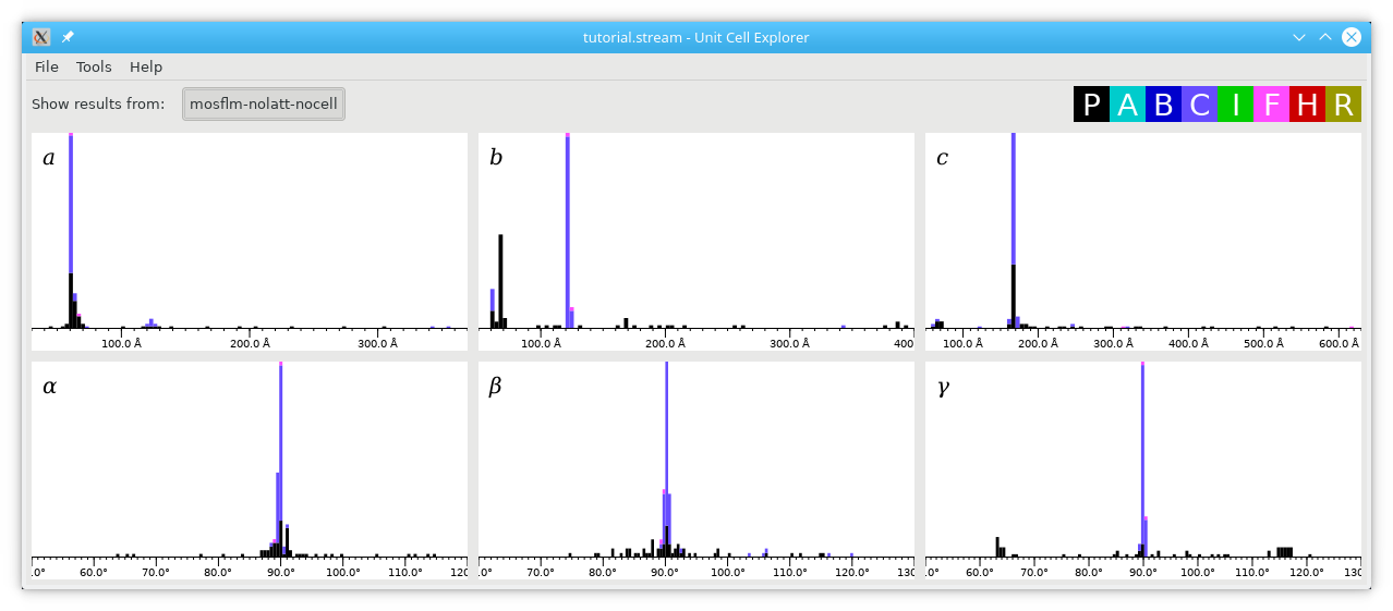
The graphs for the angles have very sharp peaks at 90 degrees, so it's clear that the unit cell is at least orthorhombic (or very close to orthorhombic). There are sharp peaks for all three of a, b and c, and the peaks are mostly purple, which corresponds (as shown in the key top right) to a C-centered cell. Note that there is a small peak in the a graph just over 120 A, which matches the large peak in the b graph. This kind of thing often happens when the axes get indexed the wrong way round by accident. Click and drag the graphs to move them around, use the scroll wheel to zoom in and out, and press the plus or minus keys to change the binning. In this way, you can examine the biggest peaks in more detail:

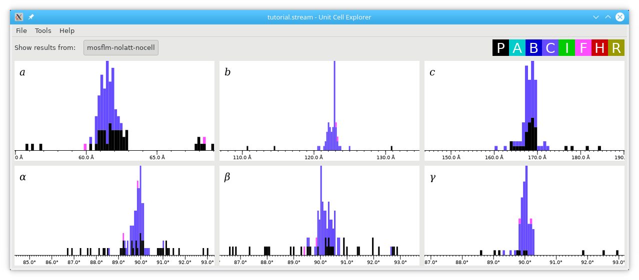
Hold down shift and click/drag to select the peaks in red, then press Ctrl+F to fit Gaussians to the peaks. This produces estimates of the unit cell parameters and the widths of their distributions:

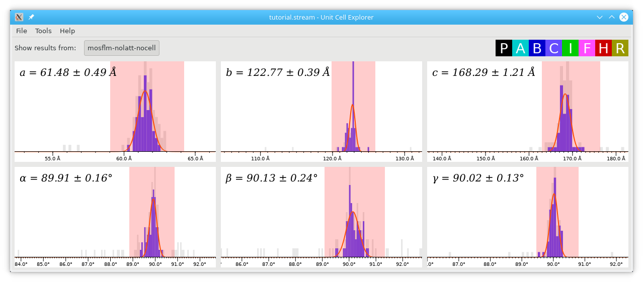
At this point, it's important to apply some crystallographic intelligence. Are the parameters selected by the indexing algorithm really the crystallographically conventional parameters for the lattice? Here are some "classic" cases to watch out for:

If you see a rhombohedral cell (all axis lengths the same, all angles the same) with an angle of 60 degrees, the lattice might in fact be cubic F.
If you see a rhombohedral cell with an angle of 109.5 degrees, the lattice might in fact be cubic I.
If the cell is monoclinic C, you will see at least three different representations of the unit cell, corresponding to the three cell choices. If you're not familiar with this, set sail for your nearest copy of the International Tables volume A, and see section 2.2.16 (in the 5th edition).
If the cell is centered (any of A, B, C, F, I or even "H"), you will almost always see at least one primitive cell which represents the same lattice.

There are, of course, many other possibilities. In this case, you can see the primitive cell appearing in black, alongside the C-centered cell in purple.

Let's proceed with the hypothesis that the lattice is orthorhombic C. Before we make our final determination of the target unit cell for indexing, we can use the lattice type information to clean up the indexing results a bit. This will be done in the next step.

8. Index the patterns using Bravais lattice information only

If you were very confident about the cell parameters determined in the previous step (or determined some other way), you could skip this step. However, it's better to work through it to make sure everything is working properly.

Even though we know the lattice parameters, it's possible to index the patterns in a more consistent way than the previous step without making use of them. Instead, we'll use only the Bravais lattice, i.e. our knowledge that the lattice is orthorhombic C. We won't tell indexamajig about the unit cell parameters themselves, so they will still not be checked for consistency.

Information about lattice types and unit cell parameters is given to CrystFEL by means of a "CrystFEL unit cell file". Simply open a text editor, and put the following lines inside it:

CrystFEL unit cell file version 1.0

lattice_type = orthorhombic
centering = C

Save the file as "5HT2B.cell" and run indexamajig again with the additional option -p 5HT2B.cell. Easy!

$ indexamajig -i files.lst -g 5HT2B-Liu-2013.geom --peaks=hdf5 --int-radius=3,4,5 -o tutorial.stream --indexing=mosflm -p 5HT2B.cell
This is what I understood your unit cell to be:
orthorhombic C, unique axis ?.
Unit cell parameters are not specified.
WARNING: Forcing --no-check-cell because reference unit cell parameters were not given.
WARNING: Forcing all indexing methods to use "-nocell", because reference cell parameters were not given.
List of indexing methods:
   0: mosflm-latt-nocell        (mosflm using Bravais lattice type as prior information)
Indexing parameters:
                  Check unit cell parameters: off
                        Check peak alignment: on
                   Refine indexing solutions: on
 Multi-lattice indexing ("delete and retry"): off
                              Retry indexing: on
   0 indexable out of    6 processed ( 0.0%),    0 crystals so far.    6 images processed since the last message.
   1 indexable out of   10 processed (10.0%),    1 crystals so far.    4 images processed since the last message.
   2 indexable out of   15 processed (13.3%),    2 crystals so far.    5 images processed since the last message.
   2 indexable out of   15 processed (13.3%),    2 crystals so far.    0 images processed since the last message.
   2 indexable out of   15 processed (13.3%),    2 crystals so far.    0 images processed since the last message.
   2 indexable out of   15 processed (13.3%),    2 crystals so far.    0 images processed since the last message.
(...)
 70 indexable out of  179 processed (39.1%),   70 crystals so far.    1 images processed since the last message.
  72 indexable out of  183 processed (39.3%),   72 crystals so far.    4 images processed since the last message.
  74 indexable out of  186 processed (39.8%),   74 crystals so far.    3 images processed since the last message.
  74 indexable out of  186 processed (39.8%),   74 crystals so far.    0 images processed since the last message.
  74 indexable out of  187 processed (39.6%),   74 crystals so far.    1 images processed since the last message.
  74 indexable out of  191 processed (38.7%),   74 crystals so far.    4 images processed since the last message.
  75 indexable out of  195 processed (38.5%),   75 crystals so far.    4 images processed since the last message.
  76 indexable out of  197 processed (38.6%),   76 crystals so far.    2 images processed since the last message.
  77 indexable out of  200 processed (38.5%),   77 crystals so far.    3 images processed since the last message.
^C
$

Once again, you only need to wait for about 100 indexed patterns.

Repeat the grep and cell_explorer parts of step 7. This time, the results should be much more consistent:

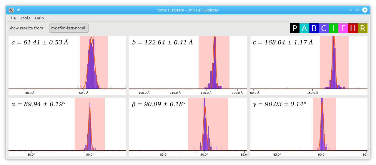
$ grep "Cell parameters" tutorial.stream
Cell parameters 29.57375 79.38331 19.61239 nm, 90.30352 90.46590 90.12323 deg
Cell parameters 6.15395 12.22018 16.78923 nm, 89.66232 90.56529 90.33316 deg
Cell parameters 6.15133 12.19475 16.61879 nm, 89.76745 89.81727 90.47255 deg
Cell parameters 6.03929 12.33804 16.80639 nm, 91.45256 91.36531 89.79536 deg
Cell parameters 6.12948 12.14581 16.60192 nm, 90.79067 90.30718 89.76016 deg
Cell parameters 6.10451 12.24309 20.84695 nm, 89.43592 87.75337 90.10239 deg
Cell parameters 6.17432 12.15292 16.69578 nm, 90.60305 89.60859 90.37155 deg
Cell parameters 6.19681 11.95545 16.71464 nm, 89.62272 91.03608 88.98001 deg
(...lots more lines...)
Cell parameters 6.16257 12.26617 16.93921 nm, 90.05327 89.71895 90.15376 deg
Cell parameters 6.16533 12.27137 17.01457 nm, 90.91694 90.42565 89.67994 deg
Cell parameters 6.17520 12.29109 16.89698 nm, 90.08418 90.92872 90.02211 deg
Cell parameters 6.17567 12.21934 16.97071 nm, 88.03281 90.62335 90.84716 deg
Cell parameters 6.17653 12.33554 16.83063 nm, 89.90496 90.34087 90.82327 deg
$ grep "lattice_type" tutorial.stream
lattice_type = orthorhombic
lattice_type = orthorhombic
lattice_type = orthorhombic
lattice_type = orthorhombic
lattice_type = orthorhombic
lattice_type = orthorhombic
lattice_type = orthorhombic
(lots more lines)
lattice_type = orthorhombic
lattice_type = orthorhombic
lattice_type = orthorhombic
lattice_type = orthorhombic
lattice_type = orthorhombic
$ grep "centering" tutorial.stream
centering = C
centering = C
centering = C
centering = C
centering = C
centering = C
centering = C
centering = C
(lots more lines)
centering = C
centering = C
centering = C
centering = C
$ cell_explorer tutorial.stream
Loaded 105 cells from 344 chunks

Note that all of the indexing results had orthorhombic C lattices (exactly what we asked it for!) and the histograms in the Unit Cell Explorer become much cleaner than before (click the image for a larger version):

9. Check and optimise the detector geometry

This is a good point at which to check and optimise the detector geometry. Even if the geometry file is supposedly correct for the experiment, it's best to check that, for example, the beam position hasn't drifted. Fortunately, CrystFEL has already done most of the work for you.

After indexing each pattern, indexamajig runs a short optimisation procedure, adjusting the unit cell parameters, orientation and beam centre position to get the best possible agreement between the observed and predicted peak locations at the same time as making sure that the observed peaks correspond to Bragg positions as closely as possible. The procedure is similar to those described by Ginn et al. and Kabsch (section 3.5.2). The required beam shift (equivalently considered as a shift of the detector) is recorded in the stream for each pattern:

$ grep "predict_refine/det_shift" tutorial.stream
predict_refine/det_shift x = -0.177 y = -0.223 mm
predict_refine/det_shift x = -0.175 y = -0.274 mm
predict_refine/det_shift x = -0.250 y = -0.208 mm
predict_refine/det_shift x = -0.062 y = -0.236 mm
predict_refine/det_shift x = -0.212 y = -0.267 mm
(lots more lines)
predict_refine/det_shift x = -0.132 y = -0.214 mm
predict_refine/det_shift x = -0.159 y = -0.220 mm
predict_refine/det_shift x = -0.081 y = -0.236 mm
predict_refine/det_shift x = -0.157 y = -0.270 mm
$

Note that there is some consistency among the values. You could plot these values with your favourite graphing software, or use the script provided with CrystFEL called detector-shift. Once again, you'll find it in the scripts folder, or download it here and mark it as executable like before. Then simply run it on the stream:

$ cp ~/crystfel/scripts/detector-shift .
$ chmod +x detector-shift
$ ./detector-shift tutorial.stream
Mean shifts: dx = -0.14 mm,  dy = -0.25 mm

A window should open, which shows the detector shifts as a scatter plot:

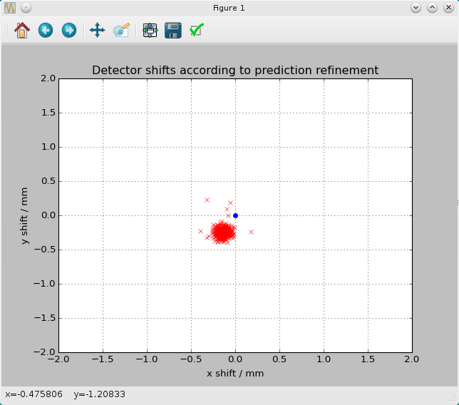
You can see that the detector position is out by about one pixel in the horizontal direction and two pixels vertically (knowing that the pixel size of the CSPAD is about 110 microns). Note that this offset has already been taken into account by the integration stages in CrystFEL, and the only reason to correct the offset is in the hope of getting a slightly higher number of indexed patterns. It's so easy to apply the offset that it's barely worth thinking about. Simply run the detector-shift script again, this time giving it your detector geometry file as well:

$ ~/crystfel/scripts/detector-shift tutorial.stream 5HT2B-Liu-2013.geom
Mean shifts: dx = -0.14 mm,  dy = -0.25 mm
Applying corrections to 5HT2B-Liu-2013.geom, output filename 5HT2B-Liu-2013-predrefine.geom
default res 9097.525473

The updated geometry file is called 5HT2B-Liu-2013-predrefine.geom, as the script tells you. Use this geometry file for further processing.

Even better geometry refinement can be performed using geoptimiser, but it's much more complicated to use, in fact there is a separate tutorial about it. The advantage of using geoptimiser is that it can refine the panel locations individually.

10. Index the patterns using unit cell parameters

The output stream from the previous step contains patterns indexed almost entirely using a consistent unit cell. However, there is still some "contamination", as you can see in the first line of the list of cell parameters above. This could be due to a second type of crystal in the mixture, but it's much more likely that it's simply a mis-indexed pattern. Before the intensities from the many patterns can be merged, we need to be sure that they're all indexed consistently. You can do this by telling indexamajig the cell parameters which it should match each pattern against.

To do this, you need to add the cell parameters to the unit cell file like this:.

CrystFEL unit cell file version 1.0

lattice_type = orthorhombic
centering = C
a = 61.40 A
b = 122.6 A
c = 168.0 A
al = 90 deg
be = 90 deg
ga = 90 deg

Note the addition of the cell parameters, which came from the Unit Cell Explorer in step 8. If you have a recent version of CrystFEL, you'll find an option to save the unit cell file directly from cell_explorer, under the File menu. However, make sure you check the contents of the file and apply the all-important crystallographic intelligence!

There is no need to update the command line, but this time we'll add -j 4 to multi-process across four CPUs, making things a bit faster. We will also switch to the updated geometry file from the previous step.

$ indexamajig -i files.lst -g 5HT2B-Liu-2013-predrefine.geom --peaks=hdf5 --int-radius=3,4,5 -o tutorial.stream --indexing=mosflm -p 5HT2B.cell -j 4
WARNING: You did not specify --int-radius.
WARNING: I will use the default values, which are probably not appropriate for your patterns.
This is what I understood your unit cell to be:
orthorhombic C, unique axis ?, right handed.
a      b      c            alpha   beta  gamma
 61.40 122.60 168.00 A     90.00  90.00  90.00 deg
a =  6.140e-09  0.000e+00  0.000e+00 m
b =  7.507e-25  1.226e-08  0.000e+00 m
c =  1.029e-24  1.029e-24  1.680e-08 m
a* =  1.629e+08 -9.973e-09 -9.973e-09 m^-1 (modulus  1.629e+08 m^-1)
b* =  0.000e+00  8.157e+07 -4.994e-09 m^-1 (modulus  8.157e+07 m^-1)
c* =  0.000e+00  0.000e+00  5.952e+07 m^-1 (modulus  5.952e+07 m^-1)
alpha* =  90.00 deg, beta* =  90.00 deg, gamma* =  90.00 deg
Cell representation is crystallographic, direct space.
List of indexing methods:
   0: mosflm-latt-cell          (mosflm using cell parameters and Bravais lattice type as prior information)
Indexing parameters:
                  Check unit cell parameters: on (axis combinations)
                        Check peak alignment: on
                   Refine indexing solutions: on
 Multi-lattice indexing ("delete and retry"): off
                              Retry indexing: on
   3 indexable out of   20 processed (15.0%),    3 crystals so far.   20 images processed since the last message.
WARNING: 1 implausibly negative reflection in cxidb-21-run0132/data1/LCLS_2013_Mar23_r0132_010315_e523.h5 (none)
  12 indexable out of   36 processed (33.3%),   12 crystals so far.   16 images processed since the last message.
  20 indexable out of   62 processed (32.3%),   20 crystals so far.   26 images processed since the last message.
  24 indexable out of   80 processed (30.0%),   24 crystals so far.   18 images processed since the last message.
  31 indexable out of   99 processed (31.3%),   31 crystals so far.   19 images processed since the last message.
(...)
2311 indexable out of 5578 processed (41.4%), 2311 crystals so far.   21 images processed since the last message.
2317 indexable out of 5601 processed (41.4%), 2317 crystals so far.   23 images processed since the last message.
2323 indexable out of 5625 processed (41.3%), 2323 crystals so far.   24 images processed since the last message.
2330 indexable out of 5646 processed (41.3%), 2330 crystals so far.   21 images processed since the last message.
2335 indexable out of 5665 processed (41.2%), 2335 crystals so far.   19 images processed since the last message.
2344 indexable out of 5687 processed (41.2%), 2344 crystals so far.   22 images processed since the last message.
2351 indexable out of 5713 processed (41.2%), 2351 crystals so far.   26 images processed since the last message.
2353 indexable out of 5736 processed (41.0%), 2353 crystals so far.   23 images processed since the last message.
2358 indexable out of 5759 processed (40.9%), 2358 crystals so far.   23 images processed since the last message.
Waiting for the last patterns to be processed...
Final: 5775 images processed, 2361 had crystals (40.9%), 2361 crystals overall.
$

This indexing run will produce the results we will merge, so let it run to completion. This is a good time to move your work to a higher performance machine, if you have one available. For example, on a single 32-core analysis node using -j 32, all 5775 patterns could be processed in about eight minutes.

Note also the use of the refined geometry file from the previous step. If you were to run detector-shift on the new script, you should see that the points in the scatter graph would cluster around the origin. Try it!

11. Evaluate the quality of the indexing

The "final" indexing yield in the previous step was 1666 out of 5775, or 29%. This is higher than the figure of 21.5% quoted by the original paper, so we're doing well! The indexing rate could possibly be increased further by using more indexing methods, for example by adding dirax-axes to the list of methods (--indexing=mosflm-axes-latt,dirax-axes). For many situations, it also helps to try MOSFLM both with and without prior lattice type information (--indexing=mosflm-axes-latt,mosflm-axes-nolatt). There are many other possibilities, depending on which programs you have available.

The indexing yield depends a lot on the quality of the patterns, and it can seem artificially low if there are many blank patterns (wrongly identified as "hits" by the hit-finder), or many low-quality patterns which are technically "hits" but not reasonably "indexable" or useful in reality.

Once indexamajig has finished, you can use the check-near-bragg script to examine the indexing results. This script works exactly like check-peak-detection, except it shows the locations of the peaks that were successfully "predicted" and integrated after indexing instead of those detected by the peak detection. Copy it from your CrystFEL distribution folder, or download it here.

$ cp ~/crystfel/scripts/check-near-bragg .
$ chmod +x check-near-bragg
$ ./check-near-bragg tutorial.stream -g 5HT2B-Liu-2013.geom
Extra arguments for hdfsee: -g 5HT2B-Liu-2013.geom
Viewing cxidb-21-run0132/data1/LCLS_2013_Mar23_r0132_010310_df17.h5
Viewing cxidb-21-run0132/data1/LCLS_2013_Mar23_r0132_010310_df11.h5
Viewing cxidb-21-run0132/data1/LCLS_2013_Mar23_r0132_010311_dfc5.h5
Viewing cxidb-21-run0132/data1/LCLS_2013_Mar23_r0132_010311_e097.h5
^C
$

Just as before, you can add extra arguments for hdfsee to the command line or edit the script to set your own defaults. Also as before, press Ctrl+C in the terminal from which you ran check-near-bragg to stop the cycle of new hdfsee windows being opened.

To evaluate the quality of the indexing, you should try to look for regions in the pattern where there are regular patterns of spots — for example lines, grids or circles — and see if the pattern of predicted spot locations (which are circled) agree with them or not. If the unit cell is small, this can be quite difficult. Don't worry if absent spots are circled at higher resolution, because indexamajig by default integrates reflections all the way to the edge of the detector regardless of the actual resolution limit of the diffraction (this behaviour can be altered if desired by using --integration=rings-rescut, or the high-resolution predictions can be removed at the merging stage).

If not many patterns could be indexed, a good course of action is to examine the peaks like in step 6, but this time looking at only the patterns which could not be indexed:

$ ./check-peak-detection --not-indexed tutorial.stream -g 5HT2B-Liu-2013.geom
Extra arguments for hdfsee: -g 5HT2B-Liu-2013.geom
Viewing cxidb-21-run0131/data1/LCLS_2013_Mar23_r0131_003712_4e09.h5
Viewing cxidb-21-run0131/data1/LCLS_2013_Mar23_r0131_003717_55a7.h5
Viewing cxidb-21-run0131/data1/LCLS_2013_Mar23_r0131_003730_684f.h5
Viewing cxidb-21-run0131/data1/LCLS_2013_Mar23_r0131_003823_b32b.h5
Viewing cxidb-21-run0131/data1/LCLS_2013_Mar23_r0131_003831_bd8d.h5
Viewing cxidb-21-run0131/data1/LCLS_2013_Mar23_r0131_003832_bead.h5
^C
$

Or, looking at only the patterns which could be indexed:

$ ./check-peak-detection --indexed tutorial.stream -g 5HT2B-Liu-2013.geom
Extra arguments for hdfsee: -g 5HT2B-Liu-2013.geom
Not showing cxidb-21-run0131/data1/LCLS_2013_Mar23_r0131_003712_4e09.h5
Not showing cxidb-21-run0131/data1/LCLS_2013_Mar23_r0131_003717_55a7.h5
Not showing cxidb-21-run0131/data1/LCLS_2013_Mar23_r0131_003730_684f.h5
Not showing cxidb-21-run0131/data1/LCLS_2013_Mar23_r0131_003823_b32b.h5
Not showing cxidb-21-run0131/data1/LCLS_2013_Mar23_r0131_003831_bd8d.h5
Not showing cxidb-21-run0131/data1/LCLS_2013_Mar23_r0131_003832_bead.h5
Not showing cxidb-21-run0131/data1/LCLS_2013_Mar23_r0131_003832_bf5b.h5
Not showing cxidb-21-run0131/data1/LCLS_2013_Mar23_r0131_003834_c195.h5
Not showing cxidb-21-run0131/data1/LCLS_2013_Mar23_r0131_003835_c2c7.h5
Not showing cxidb-21-run0131/data1/LCLS_2013_Mar23_r0131_003844_d09b.h5
Not showing cxidb-21-run0131/data1/LCLS_2013_Mar23_r0131_003851_da07.h5
Not showing cxidb-21-run0131/data1/LCLS_2013_Mar23_r0131_003900_e66d.h5
Not showing cxidb-21-run0132/data1/LCLS_2013_Mar23_r0132_010304_d69b.h5
Not showing cxidb-21-run0132/data1/LCLS_2013_Mar23_r0132_010305_d7c1.h5
Not showing cxidb-21-run0132/data1/LCLS_2013_Mar23_r0132_010306_d8bd.h5
Not showing cxidb-21-run0132/data1/LCLS_2013_Mar23_r0132_010310_deff.h5
Viewing cxidb-21-run0132/data1/LCLS_2013_Mar23_r0132_010310_df17.h5
Viewing cxidb-21-run0132/data1/LCLS_2013_Mar23_r0132_010310_df11.h5
^C
$

You might notice some trends, such as weaker patterns or poorer peak detection in the patterns which could not be indexed. In this case, you might choose to optimise the peak detection even further.

12. Check for detector saturation

An unfortunate feature of some detectors used at FEL facilities is that the dynamic range is quite small. There will probably be many saturated reflections ("overloads"), and you need to exclude these when you merge the data. Recent versions of CrystFEL include a script, called peakogram-stream, which can help you judge the maximum intensity to allow for a reflection. You can download the script here. Run it on your stream, like this:

$ ./peakogram-stream -i tutorial.stream

A graph like this should appear:

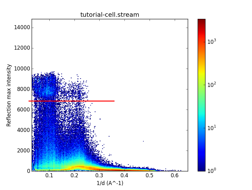
The vertical axis represents the highest pixel value in each reflection and the horizontal axis represents resolution. There is one point for every reflection in the stream, and the colour scale represents the density of points in areas where they are very concentrated. The horizontal red line has been added for illustration. See the dense "cloud" of points just above it? Those are the saturated reflections. The density is higher in the cloud because those reflections in fact have higher intensities than the detector can measure, so they appear to have lower values than they should, and get clustered around the maximum value. The reason it's a cloud and not a hard cutoff is that the images have had "pedestal" values subtracted from each pixel, and the pedestal values vary from pixel to pixel, panel to panel and even day to day. You can see, as shown by the position of the red line, that you would have to reject reflections peaking over 7000 detector units. Remember that value for the next step.

13. Merge the intensities

It's finally time to merge the intensities together! There are two ways to do this: a simple averaging-based ("Monte Carlo") method which will be described in this step, and a more advanced one which will be described in the next step.

To use simple Monte Carlo merging, simply run process_hkl on your stream, like this:

$ process_hkl -i tutorial.stream -o tutorial.hkl -y 222 --max-adu=7000
5775 images processed, 1666 crystals, 1666 crystals used.
$

Note that the saturation value, 7000, is given using --max-adu.

This will generate a new file, tutorial.hkl which contains the merged intensities. It's just a text file — you can examine it with a text editor.

The choice of point group, given to process_hkl with -y, was 222 in this example. The space group for the crystal structure in this tutorial is C222₁, which means the point group is 222. The symmetry chart has information about indexing ambiguities, which might affect the choice of point group to use for merging. Fortunately, there are no ambiguities in this example.

mmm is the point group you arrive at if you add an inversion operation to 222. Doing this means that process_hkl will treat Friedel pairs of reflections as equivalent, increasing the quality of the data but destroying any anomalous signal which may have been present. If you were definitely not interested in any anomalous signal, you could therefore use -y mmm instead. The following point group specifications can be used in CrystFEL:

Triclinic: 1, -1
Monoclinic: 2/m, 2, m
Orthorhombic: mmm, 222, mm2
Tetragonal: 4/m, 4, -4, 4/mmm, 422, -42m, -4m2, 4mm
Trigonal (rhombohedral axes): 3_R, -3_R, 32_R, 3m_R, -3m_R
Trigonal (hexagonal axes): 3_H, -3_H, 321_H, 312_H, 3m1_H, 31m_H, -3m1_H, -31m_H
Hexagonal: 6/m, 6, -6, 6/mmm, 622, -62m, -6m2, 6mm
Cubic: 23, m-3, 432, -43m, m-3m

You can append _uaX to the end of any of these point group symbols, where X is a, b or c, to use a different unique axis to the default, which is c for all the point groups where this makes sense. A common mistake is to use -y 2 with a monoclinic unit cell with "unique axis b", CrystFEL will assume that c is the unique axis by default. Use -y 2_uab in that case.

Many of the most useful figures of merit in SFX,such as the self-consistency R-factor, R_split, are calculated by splitting the patterns into two, merging each one independently, and then comparing the two resulting sets of intensities. process_hkl offers a shortcut for this purpose. The option --even-only will cause it to ignore every second crystal, and --odd-only will make it use all the crystals ignored with --even-only. Using both options, one after the other, yields the two independent sets of intensities needed for R_split:

$ process_hkl -i tutorial.stream -o tutorial.hkl1 -y 222 --max-adu=7000 --even-only
5775 images processed, 2007 crystals, 1003 crystals used.
$ process_hkl -i tutorial.stream -o tutorial.hkl2 -y 222 --max-adu=7000 --odd-only
5775 images processed, 2007 crystals, 1004 crystals used.
$

The two merged half-datasets will be called tutorial.hkl1 and tutorial.hkl2, and will be used in section 14.

14. Merge the data using scaling, partiality and post-refinement

This step assumes that you're using a recent version of CrystFEL, at least version 0.6.1.

Merging algorithms for SFX data are under intense development at the moment. The common aim of all researchers in this field is to model, as accurately as possible, the physics which give rise to the diffraction pattern and then to convert the measured intensities in each pattern directly to the underlying structure factor moduli. The more accurately the diffraction physics can be modelled and corrected for, the more accurate the measurement of the structure factor moduli should be, and hence the fewer diffraction patterns should be required for success in solving a structure. However, this is not easy! Progress has, however, recently been made, as described by Uervirojnangkoorn et al. and Ginn et al. These developments are embodied in the CrystFEL program partialator.

partialator implements scaling and post-refinement using a generalised target function, a choice of partiality models, cross-validated residuals and partiality plots, and with no external reference data set. The overall program flow is described in this paper, but some aspects have developed since then, such as the inclusion of scaling in the main refinement instead of as a separate step.

If you didn't understand any of that last paragraph, don't panic! Using partialator is almost as easy as using process_hkl. Most people can expect an improvement in data quality over that from process_hkl simply by doing the following:

$ partialator -i tutorial.stream -o tutorial.hkl -y 222 --iterations=1 --model=unity --max-adu=7000
Setting --no-pr because we are not modelling partialities (--model=unity).
5775 images loaded, 2361 crystals.
Initial partiality calculation...
Initial scaling...
Scaling: |==================================================|
Log residual went from 1.052554e+05 to 7.444357e+04, 2361 crystals
Mean B = 2.936800e-20
Scaling: |==================================================|
Log residual went from 7.885867e+04 to 7.123251e+04, 2361 crystals
Mean B = -4.627787e-20
Scaling: |==================================================|
Log residual went from 7.799002e+04 to 7.112501e+04, 2361 crystals
Mean B = -1.341730e-19
17 bad crystals:
  2344 OK
  17 B too big
Residuals:  linear          linear free     log             log free
            2.145036e+03    1.714143e+03    2.148777e+05    1.056705e+04
Scaling and refinement cycle 1 of 1
Scaling: |==================================================|
Log residual went from 7.772983e+04 to 7.099983e+04, 2344 crystals
Mean B = -2.252378e-19
Scaling: |==================================================|
Log residual went from 7.772484e+04 to 7.102961e+04, 2344 crystals
Mean B = -3.177140e-19
23 bad crystals:
  2338 OK
  23 B too big
Residuals:  linear          linear free     log             log free
            1.282511e+03    1.573327e+03    2.106331e+05    1.040949e+04
Final merge...
Scaling: |==================================================|
Log residual went from 7.764009e+04 to 7.096736e+04, 2338 crystals
Mean B = -4.104653e-19
Scaling: |==================================================|
Log residual went from 7.765026e+04 to 7.098350e+04, 2338 crystals
Mean B = -5.035855e-19
Residuals:  linear          linear free     log             log free
            1.242104e+03    1.550962e+03    2.089111e+05    1.011367e+04
Writing overall results to tutorial.hkl
Writing two-way split to tutorial.hkl1 and tutorial.hkl2
$

Most of the command line looks the same as for process_hkl, with the input stream, output file and symmetry. In addition, you have to specify which diffraction physics ("partiality") model to use (--model=unity), and how many iterations to perform of the refinement procedure which tries to maximise the agreement between the patterns by refining parameters such as the scaling factors, Debye-Waller parameters, crystal orientation and so on. The unity model actually means that no modelling should be done apart from the scaling factors and Debye-Waller parameters, so in this example we are simply performing three iterations of scaling. Nevertheless, this should still improve the data quality, which you will measure in the next step.

To try a complete modelling of the diffraction physics, change --model=unity to --model=scsphere. Since the model is now more complicated, it's not as clear that the results will always improve. Your mileage may vary, and feedback is very welcome!

Perhaps needless to say, merging using partialator requires much more memory and CPU than using process_hkl. You might want to consider running this step on a dedicated analysis machine rather than your desktop, and of course you can specify -j to increase the speed by running multiple parts of the calculation in parallel on a multi-core machine.

Finally, note that you do not need to use alternate-stream when working with partialator, because it will automatically write out tutorial.hkl1 and tutorial.hkl2 for you, each of which corresponds to half the crystals in the dataset. The half-dataset filenames will always be the same as your specified output filename, suffixed with "1" and "2" for the two halves.

15. Calculate figures of merit

Use check_hkl to calculate some simple figures of merit. You'll need to provide the unit cell file, which will be used to calculate the values in resolution shells.

$ check_hkl tutorial.hkl -y 222 -p 5HT2B.cell
Discarded 0 reflections (out of 73778) with I/sigma(I) < -inf
1/d goes from 0.287854 to 5.244288 nm^-1
overall  = 0.888138
893749 measurements in total.
73778 reflections in total.
WARNING; 2 reflections had infinite or invalid values of I/sigma(I).
Resolution shell information written to shells.dat.
$ cat shells.dat
Center 1/nm  # refs Possible  Compl       Meas   Red   SNR    Std dev       Mean     d(A)    Min 1/nm   Max 1/nm
     1.361     9692     9697  99.95     267496  27.6  4.27    3724.08    3255.93     7.35       0.287      2.436
     2.752     9647     9670  99.76     155269  16.1  1.54     814.60     466.17     3.63       2.436      3.068
     3.290     9641     9667  99.73     124941  13.0  0.44     148.67      41.07     3.04       3.068      3.512
     3.688     9667     9686  99.80     127999  13.2  0.10     141.75      11.11     2.71       3.512      3.865
     4.014     9587     9701  98.82      93836   9.8  0.06     194.34       1.28     2.49       3.865      4.163
     4.294     8854     9721  91.08      57185   6.5  0.23     566.02      -9.00     2.33       4.163      4.424
     4.541     7141     9566  74.65      34751   4.9  0.14     771.48       4.88     2.20       4.424      4.657
     4.763     5297     9729  54.45      19611   3.7 -0.11    1788.55       2.45     2.10       4.657      4.869
     4.967     3414     9693  35.22      10618   3.1 -0.20    1025.45     -23.10     2.01       4.869      5.064
     5.155      838     9631   8.70       2043   2.4  2.14    2518.91     -87.33     1.94       5.064      5.245
$

The columns are, in order from left to right: the centre of the resolution bin in inverse nanometres, the number of reflections in the resolution bin, the number of possible reflections (taking into account the point group symmetry and systematic absences due to the centering, but not the systematic absences due to glide planes and screw axes), the completeness in percent, the total number of measurements of all reflections in this bin, the mean number of measurements per reflection, the mean signal to noise ratio, the standard deviation of all the intensities in this shell, the mean of all intensities in the shell, the centre of the resolution bin in Angstroms, and finally the minimum and maximum values of 1/d for the bin in inverse nanometres.

Since CrystFEL 0.7.0, you can leave out -y 222 from all check_hkl and compare_hkl (see later) commands. The symmetry you gave to partialator or process_hkl will be used automatically.

Notice that, by default, CrystFEL integrates reflections all the way out to the edge of the detector, in the hope of bringing out very weak signals through the very large averaging process. check_hkl will divide the entire resolution range of your data up into shells, which unless your crystals consistently diffracted right to the edge of the detector probably isn't appropriate. You can restrict the resolution range to a more sensible range by using --rmin and --rmax. Both these arguments take the value of 1/d in m^-1. If you have trouble thinking in reciprocal lengths, you can also use --highres and --lowres to give values in Angstroms. From the table above, it looks like the true resolution limit is somewhere in the vicinity of 3 Angstroms, so let's look again at these figures of merit from the lowest resolution up to there. There's no need to use --lowres in this case to restrict the low resolution limit:

$ check_hkl tutorial.hkl -y 222 -p 5HT2B.cell --highres=3
Discarded 0 reflections (out of 69287) with I/sigma(I) < -inf
44641 reflections rejected because they were outside the resolution range.
1/d goes from 0.288353 to 3.332871 nm^-1
overall <snr> = 1.777141
335040 measurements in total.
24646 reflections in total.
Resolution shell information written to shells.dat.
$ cat shells.dat
Center 1/nm  # refs Possible  Compl       Meas   Red   SNR    Std dev       Mean     d(A)    Min 1/nm   Max 1/nm
     0.919     2501     2505  99.84      96579  38.6  5.24    5185.31    5150.17    10.89       0.287      1.550
     1.751     2481     2481 100.00      70685  28.5  4.15    2551.36    2252.42     5.71       1.550      1.951
     2.092     2492     2492 100.00      55019  22.1  4.16    3238.65    3325.37     4.78       1.951      2.233
     2.345     2474     2477  99.88      48972  19.8  3.30    2157.21    2076.99     4.26       2.233      2.457
     2.552     2497     2505  99.68      41020  16.4  2.08    1169.64     887.50     3.92       2.457      2.646
     2.729     2465     2470  99.80      42523  17.3  1.70     634.74     456.91     3.66       2.646      2.812
     2.886     2484     2486  99.92      40431  16.3  1.23     346.37     229.94     3.47       2.812      2.960
     3.027     2468     2476  99.68      34311  13.9  0.91     231.22     122.81     3.30       2.960      3.095
     3.156     2440     2445  99.80      33405  13.7  0.63     154.31      60.56     3.17       3.095      3.218
     3.276     2503     2507  99.84      33074  13.2  0.46     126.00      37.24     3.05       3.218      3.333
$

Note that the completeness is close to 100%, even though the number of patterns is low. check_hkl is telling you that it's measured almost all the reflections at least once, but this doesn't mean that the measurements are useful at all.

The estimated standard errors of the intensity measurements, and hence the signal to noise ratio (SNR) is estimated as described in the original CrystFEL paper. The mean and standard deviation columns in the table are the mean and standard deviations of the intensities in the resolution bin. They can sometimes be useful to spot trends in overall intensity. These numbers are not directly related to the SNR or sigma(I) values!

More useful figures or merit can be calculated by comparing the two half-datasets created in either step 12 or 13. This is done using compare_hkl, which works very similarly to check_hkl. You have to specify the two reflection lists as well as which figure of merit you want to calculate. Let's try R_split:

$ compare_hkl tutorial.hkl1 tutorial.hkl2 -y 222 -p 5HT2B.cell --fom=rsplit --highres=3
  1/d centre Rsplit/%       nref      d / A   Min 1/nm    Max 1/nm
     0.924      20.15       2458      10.83      0.297       1.550
     1.751      24.08       2454       5.71      1.550       1.951
     2.092      27.18       2458       4.78      1.951       2.233
     2.345      32.09       2407       4.26      2.233       2.457
     2.552      51.23       2349       3.92      2.457       2.646
     2.729      63.97       2380       3.66      2.646       2.812
     2.886      91.05       2377       3.47      2.812       2.960
     3.027     135.63       2291       3.30      2.960       3.095
     3.156     227.80       2257       3.17      3.095       3.218
     3.276     325.67       2320       3.05      3.218       3.333
$

R_split is quite poor for this dataset, as expected for such a small number of patterns. As a general rule, below 35% is reasonable, below 20% is good and below 10% is excellent, but these are only rough guidelines.

There are a number of other figures of merit which you can calculate using compare_hkl, such as the linear correlation coefficient (using --fom=cc), which when applied in this way would correspond to CC_1/2.You could also test for an anomalous signal by calculating CC_ano. Just for fun, let's try it now:

$ compare_hkl tutorial.hkl1 tutorial.hkl2 -y 222 -p ../5HT2B.cell --highres=3 --fom=ccano
tutorial.hkl1: 62396 reflections, resolution range 33.68 to 1.91 Angstroms (0.29691 to 5.24429 nm^-1).
tutorial.hkl2: 63012 reflections, resolution range 34.74 to 1.91 Angstroms (0.28785 to 5.23884 nm^-1).
0 reflection pairs rejected because either or both versions did not have Bijvoet partners.
2565 reflection pairs rejected because they were centric.
44626 reflection pairs accepted.
Accepted resolution range: 0.298686 to 5.054949 nm^-1 (33.48 to 1.98 Angstroms).
Relative scale factor = 0.942238, relative B factor = 1.068317 A^2
A scale factor greater than 1 means that the second reflection list is weaker than the first.
A positive relative B factor means that the second reflection list falls off with resolution more quickly than the first.
Overall CCano = 0.0241603
$ cat shells.dat
  1/d centre    CCano       nref      d / A   Min 1/nm    Max 1/nm
     0.925  0.0553656       1051      10.82      0.299       1.551
     1.751  0.0635778       1115       5.71      1.551       1.951
     2.092 -0.0041369       1131       4.78      1.951       2.233
     2.345  0.0068311       1104       4.26      2.233       2.457
     2.552 -0.0101484       1054       3.92      2.457       2.646
     2.729  0.0301614       1094       3.66      2.646       2.812
     2.886 -0.0063918       1083       3.47      2.812       2.960
     3.027 -0.0222246       1020       3.30      2.960       3.095
     3.156  0.0017413       1010       3.17      3.095       3.218
     3.276  0.0312199       1037       3.05      3.218       3.333
$

Not a convincing anomalous signal, as expected for this sample, wavelength and quantity of data.

Note that compare_hkl also accepts the --highres argument to restrict the resolution range to one that's sensible for the specific data set.

16. Export data to CCP4, XSCALE and others

The reflection lists (files ending in .hkl here, but that naming is only a convention) are also plain text, so you can almost certainly import them easily into any crystallographic software. There are scripts in the CrystFEL scripts folder for conversion into MTZ and XSCALE formats: create-mtz and create-xscale respectively. These scripts are templates for you to modify, because you need to set things like the dataset name for the MTZ file, and the space group. Download (create-mtz or create-xscale) or copy the files to your folder and edit them. To force you to edit them first, they won't run until you delete the warning at the top of the script.

$ cp ~/crystfel/scripts/create-mtz .
$ chmod +x create-mtz
$ nano create-mtz
(set dataset name, project name, lattice parameters, symmetry etc)
$ ./create-mtz tutorial.hkl
 Input: tutorial.hkl
Output: tutorial.mtz
Running 'f2mtz'...
Done.
$ cp ~/crystfel/scripts/create-xscale .
$ chmod +x create-xscale
$ nano create-xscale
(set dataset name, project name, lattice parameters, symmetry etc)
$ ./create-xscale tutorial.hkl > tutorial-xds.hkl
Unrecognised: 'CrystFEL reflection list version 2.0'
Unrecognised: 'Symmetry: 222'
Unrecognised: '   h    k    l          I    phase   sigma(I)   nmeas'
Unrecognised: 'End of reflections'
$

Note that you must redirect the output from create-xscale to a new file (tutorial-xds.hkl). You can safely ignore the "Unrecognised" messages from create-xscale — these are normal.

17. Conclusion

Congratulations! You've successfully processed a data set using CrystFEL. Now it's time to process your own data.

Your next port of call should be the manual pages, which contain comprehensive information about all of the command-line options. You should also read the best practice guidelines, which should now mostly make sense to you.

Good luck!