Error Calculation

In an experiment, the result of each measurement is slightly different due to measurement errors. Each measurement result is therefore only an approximation of the true value, or in other words: the measured value is the true, desired value with a certain error. To be able to work reasonably with the measurement results, this error should be as small as possible, the measurement result should be as close as possible to the true value.

The student experiments at Cosmic@Web measure the rate of cosmic particles $R$, i.e., the number of measured particles $N$ per time unit $t$:

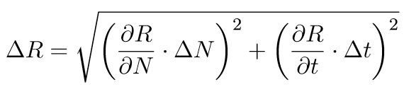
Because the rate is therefore dependent on $N$ and $t$, the error propagation law is used to calculate the measurement error $\Delta R$ (more information on this in the Wikipedia article). The formula for two independent variables, such as $N$ and $t$, is as follows:

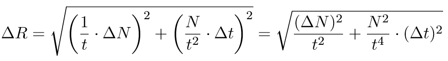
is the derivative of the function with respect to $N$, which is simply . Analogously, is the derivative with respect to $t$, it is . That's what we use and maintain:

Because the computer measures time accurately by machine, the time deviation $\Delta t$ is very small. Accordingly, the square of it $(\Delta t)$² is almost 0 and thus negligible. It remains

Now we still have to determine $\Delta N$. Natural processes like the cosmic particles showering down can be described very well with the Poisson or also Gaussian distribution. According to these mathematical laws, we can use for the deviation. Now we know how big the deviation of the measured rate is from the true value:

From this you can also determine how long you have to measure to stay below a certain error. The measurement deviation $\Delta R$ is the inaccuracy $x$ (in percent) from the true value $R$:

This formula can now be simply solved for $x$. We get

Finally, the time is determined:

By using the expected rate for $R$ and a certain error, which you want to achieve, for $x$, you can calculate the necessary measurement duration $t$. Generally, it always makes sense to measure until the error is less than 1%. How many seconds would you have to measure if a rate of 6.67 Hz is expected? Remember that the unit Hz=1/s and 1%=0.01.

With the angle measurement one calculates in a similar way. Cosmic particles reach us from all directions. However, the rate we expect for the individual directions is different. The rate depends on the angle $\alpha$, in which one measures. Therefore the formula for the calculation of the rate at the angle measurement looks as follows:

Because we simply lay the CosMO detector flat on the table for every other measurement, the measurement angle is then $\alpha$=0. With cos(0)=1, this gives exactly the simplified formula we used:

In the case of angular measurement, the rate $R$ therefore depends on three variables which are independent of each other: the number $N$, the time $t$ and the angle $\alpha$. This time the formula is accordingly:

Again, we neglect the summand with the time because it becomes almost 0. In the same way, the angle change is almost 0, so that this term also does not need to be considered further. The measurement deviation is here also:

The inaccuracy in percent is then as follows with the slightly different formula for the rate:

and the time to measure at an angle for a given error is obtained by substituting the values for the rate $R$, the error $x$ and the measurement angle $\alpha$ into the formula converted to $t$:

Errors

Exponential Functions

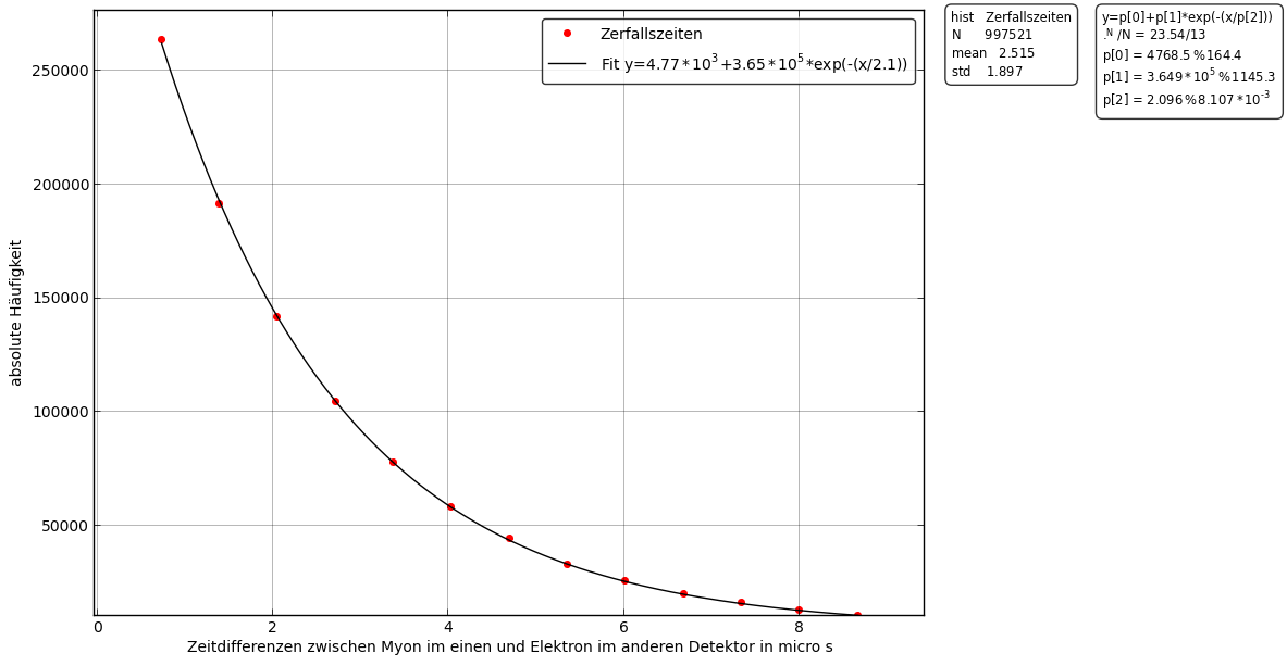
Exponential functions are mainly used to model percentage increases or decreases, multiplication times or half-lives. The general form is

The parameter $a$ influences the slope and curvature of the graph and specifies the point of intersection with the y-axis (if the graph has not been moved along the x- and y-axis).
For $\mathrm{<em>b\; >\; 1</em>}$ the curve is monotonically rising, for $\mathrm{<em>0\; <\; b\; <\; 1</em>}$ monotonically falling.

A special case is the natural or e-function $e\mathrm{^x}$, which is also displayed as $$ exp(x) .