Proposed Benchmark Case
for the simulation of csr instabilities
_________________________________________________
The Case: A simple unshielded Four-Bend Chicane
Chicane description:
The example consists of a simple four-bend chicane with parameters similar to the one required for the compression stages of the LCLS (at 5 GeV) or TESLA XFEL (at 500 MeV). It is meant to be a compromise between academic benchmarking and more practical issues. The compressor is sketched in the figure below and its parameters are shown in the first table. Click on the graphics to download a MAD input deck.
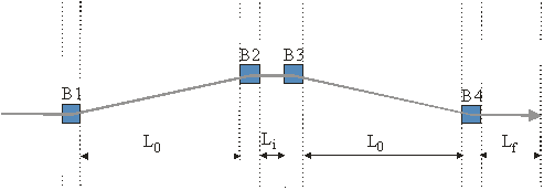
Parameters |
Symbol |
Value |
Unit |
Bend magnet length (projected) |
Lb |
0.5 |
m |
Drift length B1->B2 and B3->B4 (projected) |
L0 |
5.0 |
m |
Drift length B2->B3 |
Li |
1.0 |
m |
Post chicane drift |
Lf |
2.0 |
m |
Bend radius of each dipole magnet |
R |
10.35 |
m |
Bending Angle |
f |
2.77 |
deg |
Momentum compaction |
R56 |
-25 |
mm |
2nd order momentum compaction |
T566 |
+37.5 |
mm |
Total projected length of chicane |
Ltot |
13.0 |
m |
Vertical half gap of bends |
g |
2.5, 5 |
mm |
Note 1: Beam entrance and exit angles of the bends in degree: |
E1(B1)=0.0, E2(B1)= 2.77, E1(B2)=2.77, E2(B2)=0.0 |
|
E1(B3)=0.0, E2(B3)=-2.77, E1(B4)=-2.77,E2(B4)=0.0 |
Note 2: In the sign conventions used for R56 and T566 the bunch head is at z<0. |
Note 3: We assume hard edge magnets. The vertical gap is specified for participants interested in comparing calculations taking into account shielding effects. |
The electron beam description:
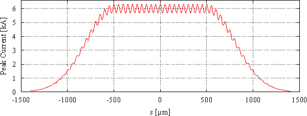
The input electron beam will have a flat top distribution with a periodic modulation of 20 wavelenghts and gaussian rise and fall (ss=30um, after compression), which are also modulated. The figure below shows an example with 5% modulation.
The simulations will be done with and without compression. The transverse phasespace is assumed to be gaussian. The beam should have a perfectly linear time-energy "chirp" (the bunch head has lower energy than the tail). Therefore the time and energy distributions will be identical. In addition a very small uncorrelated ("slice") energy spread should be added with a Gaussian distribution.
Without Compression:
Parameter |
Symbol |
Value |
Unit |
Nominal energy |
E0 |
5.0 |
GeV |
flat top current |
Q |
6 |
kA |
modulation wavelength |
l |
1, 2, 5, 10 |
um |
| relative modulation depth | h |
1*10E-3 |
|
uncorrelated relative energy spread |
(DE/E0)u-rms |
0, 4*10E-5 |
|
initial normalized rms emittance |
en,x / en,y |
0, 1, 10 / 1 |
mm-mrad |
| initial betatron functions at 1st bend entrance | bx / by |
40 / 13 |
m |
| initial alpha-function at 1st bend entrance | ax / ay |
2.6 / 1.0 |
|
With Compression:
Parameter |
Symbol |
Value |
Unit |
Nominal energy |
E0 |
5.0 |
GeV |
flat top current after compression |
Q |
6 |
kA |
modulation wavelength after compression |
l |
0.5, 1, 2, 5 |
um |
| relative modulation depth before compression | h |
1*10E-3 |
|
uncorrelated relative energy spread before compression |
(DE/E0)u-rms |
0, 4*10E-5 |
|
linear energy-z correlation |
a |
+36.0 |
m-1 |
initial normalized rms emittance |
en,x / en,y |
0, 1, 10 / 1 |
mm-mrad |
| initial betatron functions at 1st bend entrance | bx / by |
40 / 13 |
m |
| initial alpha-function at 1st bend entrance | ax / ay |
2.6 / 1.0 |
|
Note: the linear energy-z correlation is defined as: (DE/E0)(z)= (DE/E0)u-rms + a z (i.e., the bunch head (z<0) is at lower energy than the tail) |
Suggested output for comparison among the various codes
It will be helpful to look at various parameters at the end of the chicane (i.e. downstream of the 2 m drift) vs s. Such parameters are (1) the CSR-induced energy loss DE/E0 (including mean and rms), (2) the transverse kick if available, (3) the changes in position Dx and angle Dx' (including mean and rms), (4) the temporal distribution (please comment whether T566 is included or not) and (5) the normalized slice emittance.
In order to generate plots that superimpose the results of the various codes you should also provide the data as ASCII files. Items (1),(2) and (4) can be gathered in one 3-column file (col. 1: s in um, col. 2: I in kA, col. 3: DE/E0). Item (3) should be provided in a separated file 3-column file (col. 1: x in um, col. 2: Dx in um, col. 3: Dx' in urad). Item (5) should be provided in a 2-column file (col. 1: s in um, col. 2: ex in mm mrad). These are the same parameters we want to compare for the CSR benchmarking from the CSR Workshop 2002. Additionally a gain curve should be created from the different modulation cases.