Remarks: Adapated to formatting with Doxygen (C. Kleinwort, DESY, 2012). The abstract has been moved to section Introduction. Some clarifications as result of user feedback included (C. Kleinwort, DESY, 2013). A list of major changes to the implementation described in this manual can be found here. The solution method GMRES described later has never been implemented. Instead MINRES can be used.

Preface

Linear least squares problems. The most important general method for the determination of parameters from measured data is the linear least squares method. It is usually stable and accurate, requires no initial values of parameters and is able to take into account all the correlations between different parameters, even if there are many parameters.

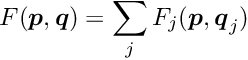
Global and local parameters. The parameters of a least squares problem can sometimes be distinguished as global and local parameters. The mathematical model underlying the measurement depends on both types of parameters. The interest is in the determination of the global parameters, which appear in all the measurements. There are many sets of local parameters, where each set appears only in one, sometimes small, subset of measurements.

Alignment of large detectors in particle physics. Alignment problems for large detectors in particle physics often require the determination of a large number of alignment parameters, typically of the order of to $1\,000$ , but sometimes above $10\,000$ . Alignment parameters for example define the accurate space coordinates and orientation of detector components. In the alignment usually special alignment measurements are combined with data of particle reaction, typically tracks from physics interactions and from cosmics. In this paper the alignment parameters are called global parameters. Parameters of a single track like track slopes and curvatures are called local parameters.

One approximate alignment method is to perform least squares fits on the data e.g. of single tracks assuming fixed alignment parameters. The residuals, the deviations between the fitted and measured data, are then used to estimate the alignment parameters afterwards. Single fits depend only on the small number of local parameters like slope or curvature of the track, and are easy to solve. This approximate method however is not a correct method, because the (local) fits depend on a wrong model, they ignore the global parameters, and the result are biased fits. The adjustment of parameters based on the observed (biased) residuals will then result in biased alignment parameters. If these alignment parameters are applied as corrections in repeated fits, the remaining residuals will be reduced, as desired. However, the fitted parameters will still be biased. In practice this procedure is often applied iteratively; it is however not clear wether the procedure is converging.

A more efficient and faster method is an overall least squares fit, with all the global parameters and local parameters, perhaps from thousands or millions of events, determined simultaneously. The Millepede algorithm makes use of the special structure of the least squares matrices in such a simultaneous fit: the global parameters can be determined from a matrix equation, where the matrix dimension is given by the number of global parameters only, irrespective of the total number of local parameters, and without any approximation. If is the number of global parameters, then an equation with a symmetric -by- matrix has to be solved. The Millepede programm has been used for up to $n \approx 5000$ parameters in the past. Solution of the matrix equation was done with a fast program for the solution of matrix equations with inversion of the symmetric matrix, which on a standard PC takes a time $t \approx 2 \times 10^{-8} \, \textrm{sec}\, \times n^3$ . Even for the computing time is, with $t = 2 \times 10^{-8} \, \textrm{sec}\, \times 5000^3 = 40$ minutes, still acceptable.

The next-generation detectors in particle physics however require up to about 100000 global parameters and with the previous solution method the space- and time-consumption is too large for a standard PC. Memory space is needed for the full symmetric matrix, corresponding to $1/2 n^2 \times 8$ bytes for double precision, if the symmetry of the matrix is observed, and if solution is done in-space. This means memory space of 400 Mbyte and 40 Gbyte for $n = 10\,000$ and $n = 100\,000$ , and computing times of about 6 hours and almost a year, respectively.

Millepede I and II. The second version of the Millepede programm, described here, allows to use several different methods for the solution of the matrix equation for global parameters, while keeping the algorithm, which decouples the determination of the local parameters, i.e. still taking into account all correlations between all global parameters. The matrix can be stored as a sparse matrix, if a large fraction of off-diagonal elements has zero content. A complete matrix inversion of a large sparse matrix would result in a full matrix, and would take an unacceptable time. Different methods can be used in Millepede II for a sparse matrix. The symmetric matrix can be accumulated in a special sparse storage scheme. Special solution methods can be used, which require only products of the symmetric sparse matrix with different vectors. Depending on the fraction of vanishing matrix elements, solutions for up to a number of 100000 global parameters should be possible on a standard PC.

The structure of Millepede II is different from the Millepede I version. The accumulation of data and the solution are splitted, with the solution in a stand-alone program. Furthermore the global parameters are now characterized by a label (any positive integer) instead of a (continuous) index. Those features should simplify the application of the program for alignment problems even for large number of global parameters in the range of .

Mathematical Methods

Large problems with global and local parameters

The solution of optimization problems requires the determination of certain parameters. In certain optimization problems the parameters can be classified as either global or local. This classification can be used, when the input data of the optimization problem consist out of a potentially large group of data sets, where the description of each single set of data requires certain local parameters, which appear only in the description of one data set. The global parameter may appear in all data sets, and the interest is in the determination of these global parameters. The local parameters can be called nuisance parameters.

An example for an optimization problem with global and local parameters from experimental high energy physics is the alignment of track detectors using a large number of track data. The track data are position measurements of a charged particle track, which can be fitted for example by a helix with five parameters, if the track detector is in a homogeneous magnetic field. The position measurement, from several detector planes of the track detector, depend on the position and orientation of certain sensors, and the corresponding coordinates and angles are global parameters. In an alignment the values of the global parameters are improved by minimizing the deviations between measurement and parametrization of a large number of tracks. Numbers of tracks in the order of one Million, with of the order of 10 data poinst per track, and of to global parameters are typical for modern track detectors in high energy physics.

Optimal values of the global parameters require a simultaneous fit of all parameters with all data sets. A straight-forward ansatz for such a fit seems to require to fit Millions of parameters, which is impossible. An alternative is to perform each local fit separately, fitting the local parameters only. From the residuals of the local fits one can then try to fit the values of the global parameters. This approach neglects the correlations between the global and local parameters. Nevertheless the method can be applied iteratively with the hope, that the convergence is not to slow and does not require too many iterations.

The optimization problem is complicated by the fact, that often not all global parameters are defined by the ansatz. In the alignment example the degrees of freedom describing a translation and rotation of the whole detector are not fixed. The solution of the optimization problem requires therefore certain equality constraints, for example zero overall translation and rotation of the detector; these constraints are described by a linear combination of global parameters. Such an equality constraint can only be satisfied in an overall fit, not with separated local and global fits.

Note: Constraints in optimization are either equality or inequality constraints, which have exactly to be taken into account in the solution. The term constraint is often used in a loose sense, like: `‘the parameters are constrained by our measurement’'.

Global parameters are denoted by the vector $\Vek{p}$ and local parameters for the data set by the vector $\Vek{q}_j$ . The objective function to be minimized in the global parameter optimization is the sum of the local objective Function, depending on the global parameters $\Vek{p}$ and the vectors $\Vek{q}_j$ :

$\begin{equation*} F(\Vek{p}, \Vek{q}) = \sum_j F_j(\Vek{p}, \Vek{q}_j) \end{equation*}$

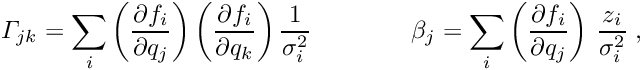
In the least squares method the objective function to be minimized is a sum of the squares of residuals between the measured values and the parametrization, weighted by the inverse variance of the measured value:

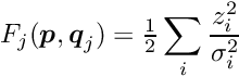
$\begin{equation*} F_j(\Vek{p}, \Vek{q}_j) = \tfrac{1}{2} \sum_i \frac{z_i^2}{\sigma_i^2} \end{equation*}$

with the residual $z_i = y_i - f_i(\Vek{p},\Vek{q}_j)$ , where is the measured value and $f_i(\Vek{p},\Vek{q}_j)$ is the corresponding parametrization. This form of the objective function assumes independent measurements, with a single variance value $\sigma_i$ assigned.

Note: In experimental high energy physics the objective function is usually called a $\chi^2$ -function. In statistics there is a $\chi^2$ -distribution with a well-defined meaning. The minimum value $\times 2$ of the objective function follows, under certain conditions, the $\chi^2$ -distribution.

Optimization without constraints

The quadratic model

The standard optimization method for smooth objective functions is the Newton method. The objective function $F(\Vek{p})$ , depending on a parameter vector $\Vek{p}$ , is approximated by a quadratic model $\tilde{F}(\Vek{p})$

$\begin{equation*} \label{eq:qapp} \tilde{F}_k \left( \Vek{p}_k + \Vek{d} \right) = F_k + \Vek{g}\trans \Vek{d} + \tfrac{1}{2} \Vek{d}\trans \Vek{C} \Vek{d} \end{equation*}$

where $\Vek{p}_k$ is the vector $\Vek{p}$ in the -th iteration and where the vector $\Vek{g}$ is the gradient of the objective function; the matrix $\Vek{C}$ is the Hessian (second derivative matrix) of the objective function $F(\Vek{p})$ or an approximation of the Hessian. The minimum of the quadratic approximation requires the gradient to be equal to zero. A step $\Vek{d}$ in parameter space is calculated by the solution of the matrix equation, obtained from the derivative of the quadratic model:

(1)

$\begin{equation*} \label{eq:cdmg} \Vek{C} \, \Vek{d} = - \Vek{g} \, . \end{equation*}$

With the correction vector $\Vek{d}$ the new value $\Vek{p}_{k+1} = \Vek{p}_k + \Vek{d}$ for the next iteration is obtained. The matrix $\Vek{C}$ is a constant in a linear least squares problem and the minimum is determined in a single step (no iteration necessary).

Partitioning of matrices

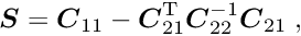
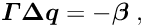
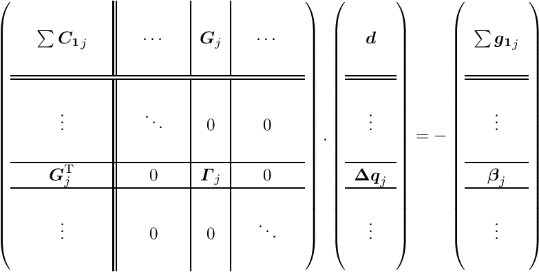
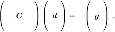
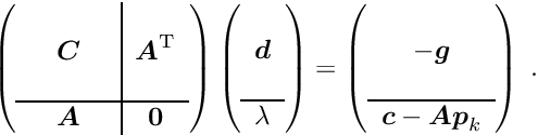
The special structure of the matrix $\Vek{C}$ in a matrix equation $\Vek{C} \Vek{d} = - \Vek{g}$ may allow a significant simplification of the solution. Below the symmetric matrix $\Vek{C}$ is partitioned into submatrices, and the vectors $\Vek{d}$ and $\Vek{g}$ are partitioned into two subvectors; then the matrix equation can be written in the form

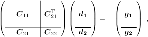
$\begin{equation*} \left( \begin{array}{ccc|c} & & & \\ & \Vek{C}_{11} & & \Vek{C}_{21}\trans \\ & & & \\ \hline & \Vek{C}_{21} & & \Vek{C}_{22} \end{array} \right) \left( \begin{array}{c} ~\\ \Vek{d_1} \\ ~\\ \hline \Vek{d_2} \end{array} \right) = - \left( \begin{array}{c} ~\\ \Vek{g_1} \\ ~\\ \hline \Vek{g_2} \end{array} \right) \; , \end{equation*}$

where the submatrix $\Vek{C}_{11}$ is a -by- square matrix and the submatrix $\Vek{C}_{22}$ is a -by- square matrix, with , and $\Vek{C}_{21}$ is a -by- matrix. Now it is assumed that the inverse of the -by- sub-matrix $\Vek{C}_{22}$ is available. In certain problems this may be easily calculated, for example if $\Vek{C}_{22}$ is diagonal.

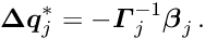
If the sub-vector $\Vek{d}_1$ would not exist, the solution for the sub-vector $\Vek{d}_2$ would be defined by the matrix equation 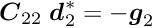$\Vek{C}_{22} \; \Vek{d}_2^{*} = - \Vek{g}_2$ , where the star indicates the special character of this solution, which is

(2)

$\begin{equation*} \label{eq:spa2} \Vek{d_2}^{*} = - \Vek{C}_{22}^{-1} \; \Vek{g_2} \; . \end{equation*}$

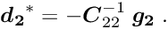
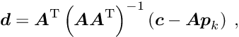
Now, having the inverse sub-matrix $\Vek{C}_{22}^{-1}$ , the submatrix of the complete inverse matrix $\Vek{C}$ correponding to the upper left part $\Vek{C}_{11}$ is the inverse of the symmetric -by- matrix

(3)

$\begin{equation*} \label{eq:Schur} \Vek{S} = \Vek{C}_{11} - \Vek{C}_{21}\trans \Vek{C}_{22}^{-1} \Vek{C}_{21} \; , \end{equation*}$

the so-called Schur complement. With this matrix $\Vek{S}$ the solution of the whole matrix equation can be written in the form

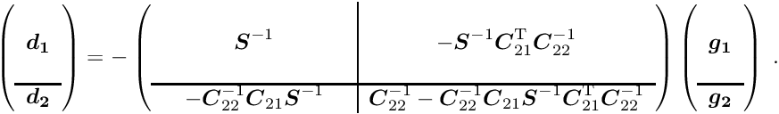
$\begin{equation*} \label{eq:solvea1} \left( \begin{array}{c} ~\\ \Vek{d_1} \\ ~\\ \hline \Vek{d_2} \end{array} \right) = - \left( \begin{array}{ccc|c} & & & \\ & \Vek{S}^{-1} & & - \Vek{S}^{-1} \Vek{C}_{21}\trans \Vek{C}_{22}^{-1} \\ & & & \\ \hline & - \Vek{C}_{22}^{-1} \Vek{C}_{21} \Vek{S}^{-1} & & \Vek{C}_{22}^{-1} - \Vek{C}_{22}^{-1} \Vek{C}_{21} \Vek{S}^{-1} \Vek{C}_{21}\trans \Vek{C}_{22}^{-1} \end{array} \right) \left( \begin{array}{c} ~\\ \Vek{g_1} \\ ~\\ \hline \Vek{g_2} \end{array} \right) \; . \end{equation*}$

The sub-vector $\Vek{d_1}$ can be obtained from the solution of the matrix equation

(4)

$\begin{equation*} \label{eq:solvea2} \left( \begin{array}{ccc} & & \\ & \Vek{C}_{11} - \Vek{C}_{21}\trans \Vek{C}_{22}^{-1} \Vek{C}_{21} \\ & & \end{array} \right) \left( \begin{array}{c} ~\\ \Vek{d_1} \\ ~\\ \end{array} \right) = - \left( \begin{array}{c} ~\\ \Vek{g_1} - \Vek{C}_{21}\trans \Vek{C}_{22}^{-1} \Vek{g}_2 \\ ~\\ \end{array} \right) =- \left( \begin{array}{c} ~\\ \Vek{g_1} - \Vek{C}_{21}\trans \Vek{d_2}^* \\ ~\\ \end{array} \right) \end{equation*}$

using the known right-hand-side of the equation with the special solution $\Vek{d_2}^*$ .

In a similar way the vector $\Vek{d_2}$ could be calculated. However, if the interest is the determination of this sub-vector $\Vek{d_1}$ only, while the sub-vector $\Vek{d_2}$ is not needed, then only the equation (4) has to be solved after calculation of the special solution $\Vek{d_2}^*$ (equation (2)) and the Schur complement $\Vek{S}$ (equation (3)). Some computer time can be saved by this method, especially if the matrix $\Vek{C}_{22}^{-1}$ is easily calculated or already known before; note that the matrix $\Vek{C}_{22}$ does not appear directly in the solution, only the inverse $\Vek{C}_{22}^{-1}$ .

This method of removing unnecessary parameters was already known in the nineteenth century. The method can be applied repeatedly, and therefore may simplify the solution of problems with a large number of parameters. The method is not an approximation, but is exact and it takes into account all the correlations introduced by the removed parameters.

Note: One example is: Schreiber, O. (1877): Rechnungsvorschriften für die trigonometrische Abteilung der Landesaufnahme, Ausgleichung und Berechnung der Triangulation zweiter Ordnung. Handwritten notes. Mentioned in W. Jordan (1910): Handbuch der Vermessungskunde, Sechste erw. Auflage, Band I, Paragraph III: 429-433. J.B.Metzler, Stuttgart.

Local parameters

A set of local measured data is considered. The local data are assumed to be described by a linear or non-linear function $f(x_i,\Vek{q})$ , depending on a (small) number of local parameters $\Vek{q}$ .

$\begin{equation*} \label{eq:measur} y_i = f(x_i,\Vek{q}) + \varepsilon_i \; . \end{equation*}$

The parameters $\Vek{q}$ are called the local parameters, valid for the specific group of measurements (local-fit object). The quantity $\varepsilon$ is the measurement error, with standard deviation $\sigma_i$ . The quantity is assumed to be the coordinate of the measured value , and is one argument of the function $f(x_i,\Vek{q})$ .

The local parameters are determined in a least squares fit. If the function $f(x_i,\Vek{q})$ depends non-linearly on the local parameters $\Vek{q}$ , an iterative procedure is used, where the function is linearized, i.e. the first derivatives of the function $f(x_i,\Vek{q})$ with respect to the local parameters $\Vek{q}$ are calculated. The function is thus expressed as a linear function of local parameter corrections $\Vek{\D q}$ at some reference value $\Vek{q}_k$ :

(5)

$\begin{equation*} \label{eq:ydeff} f(x_i,\Vek{q}_k +\Vek{\D q}) = f(x_i,\Vek{q}_k) + \frac{\partial f}{\partial q_1} \D q_1 + \frac{\partial f}{\partial q_2} \D q_2 + \ldots \; , \end{equation*}$

where the derivatives are calculated for $\Vek{q} \equiv \Vek{q}_k$ . For each single measured value, the residual measurement

$\begin{equation*} z_i \equiv y_i - f(x_i,\Vek{q}_k) \end{equation*}$

is calculated. For each iteration a linear system of equations (normal equations of least squares) has to be solved for the parameter corrections $\Vek{\D q}$ with a matrix $\Vek{\Gamma}$ and a gradient vector $\Vek{g}$ with elements

(6)

$\begin{equation*} \label{eq:normaloc} \Gamma_{jk} = \sum_i \left( \frac{\partial f_i}{\partial q_j} \right) \left( \frac{\partial f_i}{\partial q_k} \right) \frac{1}{\sigma_i^2} \quad \quad \quad \quad \beta_j= \sum_i \left( \frac{\partial f_i}{\partial q_j} \right) \, \frac{z_i}{\sigma_i^2} \; , \end{equation*}$

where the sum is over all measurements of the local-fit object. Corrections $\Vek{\D q}$ are determined by the solution of the matrix equation

$\begin{equation*} \Vek{\Gamma} \Vek{\D q} = - \Vek{\beta} \; , \end{equation*}$

and a new reference value is obtained by

$\begin{equation*} \Vek{q}_{k+1} = \Vek{q}_k + \Vek{\D q} \end{equation*}$

and then, with increased by 1, this is repeated until convergence is reached.

Global parameters

Now global parameters are considered, which contribute to all the measurements. The expectation function (5) is extended to include corrections for global parameters. Usually only few of the global parameters influence a local-fit object. A global parameter is identified by a label $\ell$ ; assuming that labels $\ell$ from a set $\Omega$ contribute to a single measurement the extended equation becomes

$\begin{equation*} \label{eq:zdefey} z_i = y_i - f(x_i,\Vek{q},\Vek{p}) = \sum_{j=1}^{\nu} \left( \frac{\partial f}{\partial q_j} \right) \D q_j + \sum_{\ell \in \Omega} \left( \frac{\partial f}{\partial p_{\ell}} \right) \D p_{\ell} \; . \end{equation*}$

The simultaneous fit of global and local parameters

In the following it is assumed that there is a set of local measurements. Each local measurement, with index , depends on $\nu$ local parameters $\Vek{q}_j$ , and all of them depend on the global parameters. In a simultaneous fit of all global parameters plus local parameters from subsets of the data there are in total 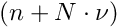$(n+N\cdot\nu)$ parameters, and the standard solution requires the solution of $(n+N\cdot\nu)$ equations with a computation proportional to $(n+N \cdot \nu)^3$ . In the next chapter it is shown, that the problem can be reduced to a system of equations, for the global parameters only.

For a set of local measurements one obtains a system of least squares normal equations with large dimensions, as is shown in equation (7) The matrix on the left side of equation (7) has, from each local measurement, three types of contributions. The first part is a contribution of a symmetric matrix $\Vek{C_1}_j$ , of dimension (number of global parameters), and is calculated from the (global) derivatives $\partial f/\partial p_{\ell}$ . All the matrices $\Vek{C_1}_j$ are added up in the upper left corner of the big matrix of the normal equations. The second contribution is the symmetric matrix $\Vek{\Gamma}_j$ (compare equation (6)), which gives a contribution to the big matrix on the diagonal and is depending only on the -th local measurement and the (local) derivatives $\partial f/\partial q_j$ . The third (mixed) contribution is a rectangular matrix $\Vek{G}_j$ , with a row number of (global) and a column number of $\nu$ (local). There are two contributions to the vector of the normal equations (gradient), $\Vek{g_1}_j$ for the global and $\Vek{\beta}_j$ for the local parameters. The complete matrix equation is given by

(7)

$\begin{equation*} \label{eq:huge} \renewcommand{\arraystretch}{1.2} \left( \begin{array}{ccc||ccc|c|ccc} & & & & & & & & & \\ & \sum \Vek{C_1}_j & & & \cdots & & \Vek{G}_j & & \cdots & \\ & & & & & & & & & \\ \hline \hline & & & & & & & & & \\ & \vdots & & & \ddots & & 0 & & 0 & \\ & & & & & & & & & \\ \hline & \Vek{G}\trans_j & & & 0 & & \Vek{\Gamma}_j & &0 & \\ \hline & & & & & & & & & \\ & \vdots & & & 0 & & 0 & & \ddots & \\ & & & & & & & & & \\ \end{array} \right) . \left( \begin{array}{c} \\ \Vek{d} \\ \\ \hline \hline \\ \vdots \\ \\ \hline \Vek{\D q}_j \\ \hline \\ \vdots \\ \\ \end{array} \right) = - \left( \begin{array}{c} \\ \sum \Vek{g_1}_j \\ \\ \hline \hline \\ \vdots \\ \\ \hline \Vek{\beta}_j \\ \hline \\ \vdots \\ \\ \end{array} \right) \end{equation*}$

In this matrix equation the matrices $\Vek{C_1}_j$ , $\Vek{\Gamma}_j$ , $\Vek{G}_j$ and the vectors $\Vek{g_1}_j$ and $\Vek{\beta}_j$ contain contributions from the -th local measurement. Ignoring the global parameters (i.e. keeping them constant) one could solve the normal equations 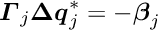$\Vek{\Gamma}_j \Vek{\D q}_j^* = - \Vek{\beta}_j$ for each local measurement separately by

$\begin{equation*} \label{eq:ignore} \Vek{\D q}_j^* = - \Vek{\Gamma}_j^{-1} \Vek{\beta}_j \, . \end{equation*}$

The complete system of normal equations has a special structure, with many vanishing sub-matrices. The only connection between the local parameters of different partial measurements is given by the sub-matrices $\Vek{G}_j$ und $\Vek{C_1}_j$ ,

Reduction of matrix size

The aim of the fit is solely to determine the global parameters; final best parameters of the local parameters are not needed. The matrix of equation (7) is written in a partitioned form. The general solution can also be written in partitioned form. Many of the sub-matrices of the huge matrix in equation (7) are zero and this has the effect, that the formulas for the sub-matrices of the inverse matrix are very simple.

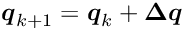
By this procedure the normal equations

(8)

$\begin{equation*} \label{eq:nsb} \renewcommand{\arraystretch}{1.2} \left( \begin{array}{ccc} & & \\ & \Vek{C} & \\ & & \\ \end{array} \right) \left( \begin{array}{c} \\ \Vek{d} \\ \\ \end{array} \right) = - \left( \begin{array}{c} \\ \Vek{g} \\ \\ \end{array} \right) \; , \end{equation*}$

are obtained, which only contain the global parameters, with a modified matrix $\Vek{C}$ and a modified vector $\Vek{g}$ ,

$\begin{equation*} \label{eq:nsc} \Vek{C} = \sum_j \Vek{C_1}_j + \sum_j \Vek{C_2}_j \quad \quad \quad \quad \Vek{g} = \sum_j \Vek{g_1}_j + \sum_j \Vek{g_2}_j \end{equation*}$

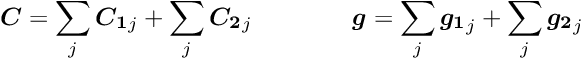
with the following local contributions to $\Vek{C}$ and $\Vek{g}$ from the -th local fit:

(9)

$\begin{equation*} \label{eq:nsc2} \Vek{C_2}_j = - \Vek{G}_j \Vek{\Gamma}_j^{-1} \Vek{G}_j\trans \quad \quad \quad \quad \Vek{g_2}_j = - \Vek{G}_j \left( \Vek{\Gamma}_j^{-1} \Vek{\beta}_j\right) = - \Vek{G}_j \Vek{\D q}_j^* \; . \end{equation*}$

The set of normal equations (8) contains explicitly only the global parameters; implicitly it contains, through the correction matrices, the complete information from the local parameters, influencing the fit of the global parameters. The parentheses in equation (9) represents the solution for the local parameters, ignoring the global parameters. The solution

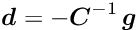
$\begin{equation*} \label{eq:ared} \Vek{d} = - \Vek{C}^{-1}\, \Vek{g} \end{equation*}$

represents the solution vector $\Vek{d}$ with covariance matrix $\Vek{C}^{-1}$ . The solution is direct, no iterations or approximations are required. The dimension of the matrix to compute $\Vek{d}$ from equation (1) is reduced from $(n+N\cdot\nu)$ to . The vector $\Vek{d}$ is the correction for the global parameter vector $\Vek{p}$ . Iterations may be necessary for other reasons, namely

the equations depend non-linearly on the global parameters; the equations have to be linearized;
the data contain outlier, which have to be removed in a sequence of cuts, becoming narrower during the iteration, or which have to be down-weighted;
the accuracy of the data is not known before, and has to be determined from the data (after the alignment).

For iterations the vector $\Vek{d}$ is the correction for the global parameter vector $\Vek{p}_k$ in iteration to obtain the global parameter vector $\Vek{p}_{k+1} = \Vek{p}_k + \Vek{d}$ for the next iteration.

Nonlinear least squares

A method for linear least squares fits with a large number of parameters, perhaps with linear constraints, is discussed in this paper. Sometime of course the model is nonlinear and also constraints may be nonlinear. The standard method to treat these problems is linearization: the nonlinear equation is replaced by a linear equation for the correction of a parameter (Taylor expansion); this requires a good approximate value of the parameter. In principle this method requires an iterative improvement of the parameters, but sometimes even one iteration may be sufficient.

The treatment of nonlinear equations is not directly supported by the program package, but it will in general not be too difficult to organize a program application with nonlinear equations.

Outliers

Cases with very large residuals within the data can distort the result of the method of least squares. In the method of M-estimates, the least squares method is modified to Maximum likelihood method. Basis is the residual between data and function value (expected data value), normalized by the standard deviation:

$\begin{equation*} \zeta = \frac{y - f(x)}{\sigma} \end{equation*}$

In the method of M-estimates the objective function to be minimized is defined in terms of a probability density function of the normalized residual

$\begin{equation*} F(.) = \sum_i \rho(\zeta_i) \quad \quad \quad \quad \rho(\zeta) = \ln \textrm{pdf}(\zeta) \end{equation*}$

From the probability density function $\textrm{pdf}(\zeta)$ a influence function $\psi(\zeta)$ is defined

$\begin{equation*} \textrm{influence function} \; \psi(\zeta) = \dd \rho(\zeta)/\dd \zeta \quad \quad \quad \quad \textrm{additional weight factor} \; \omega(\zeta) = \psi(\zeta)/\zeta \end{equation*}$

and a weight in addition to the normal least squares weight $w_i = 1/\sigma_i^2$ can be derived from the influence function for the calculation of the (modified) normal equations of least squares.

For the standard least squares method the function $\rho(\zeta)$ is simply $\rho(\zeta) = \zeta^2/2$ and it follows, that the influence function is $\psi(\zeta)=\zeta$ and the weight factor is $\omega(\zeta) = 1$ (i.e. no extra weight). The influence function value increases with the value of the normalized residual without limits, and thus outliers have a large and unlimited influence. In order to reduce the influence of outliers, the probability density function $\textrm{pdf}(\zeta)$ has to be modified for large values of $|\zeta|$ to avoid the unlimited increase of the influence. Several functions $\textrm{pdf}(\zeta)$ are proposed, for example the Huber function and the Cauchy function.

Huber function: A simple function is the Huber function, which is quadratic and thus identical to least squares for small $|\zeta|$ , but linear for larger $|\zeta|$ , where the influence function becomes a constant $C_{\textrm{H}} \cdot \textrm{sign}(\zeta)$ :

$\begin{equation*} \label{eq:huber} \textrm{Huber function: pdf} \quad \rho(\zeta) = \begin{cases} \zeta^2/2 \\ C_{\textrm{H}} \left( |\zeta| - C_{\textrm{H}}/2 \right) \\ \end{cases} \quad \quad \textrm{factor} \quad \omega(\zeta) = \begin{cases} 1 &\textrm{if} \; |\zeta| \le C_{\textrm{H}} \\ C_{\textrm{H}}/|\zeta| &\textrm{if} \; |\zeta| > C_{\textrm{H}} \end{cases} \end{equation*}$

The extra weight is $\omega(\zeta) = C_{\textrm{H}}/|\zeta|$ for large $|\zeta|$ . A standard value for $C_{\textrm{H}}$ is $C_{\textrm{H}}=1.345$ ; for this value the efficiency for Gaussian data without outliers is still 95 %. For very large deviations the additional weight factor decreases with $1/|\zeta|$ .

Cauchy function: For small deviation the Cauchy function is close to the least squares expression, but for large deviations it increases only logarithmically. For very large deviations the additional weight factor decreases with $1/\zeta^2$ :

$\begin{equation*} \label{eq:cauchy} \textrm{Cauchy function: pdf} \quad \rho(\zeta) = \tfrac{1}{2} C_{\textrm{c}} \ln \left( 1 + \left( \zeta/ C_{\textrm{c}}\right)^2 \right) \quad \quad \quad \textrm{factor} \quad \omega = 1/\left( 1 + \left( \zeta/ C_{\textrm{c}} \right)^2 \right) \end{equation*}$

A standard value is $C_{\textrm{c}}=2.3849$ ; for this value the efficiency for Gaussian data without outliers is still 95 %.

Optimization with linear constraints

The minimization of an objective function $F(\Vek{p})$ is often not sufficient. Several degrees of freedom may be undefined and require additional conditions, which can be expressed as equality constraints. For linear equality constraints the problem is the minimization of a non-linear function $F(\Vek{p})$ subject to a set of linear constraints:

$\begin{equation*} \label{eq:cproblem} \min F(\Vek{p}) \quad \quad \quad \textrm{subject to} \; \Vek{A} \Vek{p} = \Vek{c} \; , \end{equation*}$

where $\Vek{A}$ is a -by- matrix and $\Vek{c}$ is a -vector with $m \le n$ . In iterative methods the parameter vector $\Vek{p}$ is expressed by 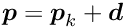$\Vek{p} = \Vek{p}_k + \Vek{d}$ with the correction $\Vek{d}$ to $\Vek{p}_k$ in the -th iteration, satisfying the equation

$\begin{equation*} \Vek{A} \left( \Vek{p}_k + \Vek{d} \right) = \Vek{c} \end{equation*}$

with $\Vek{p}_{k+1} = \Vek{p}_k + \Vek{d}$ .

There are two methods for linear constrainst:

in the Lagrange multiplier method additional parameters are introduced and the linear system of unknowns has to be solved;
by elimination the minimization problem with constraints is transformed to an unconstrained problem with unknowns. However the sparsity of a matrix may be destroyed by the elimination.

The Lagrange method is used in Millepede.

The Lagrange multiplier method

In the Lagrange multiplier method one additional parameter $\lambda$ is introduced for each single constraint, resulting in an -vector $\Vek{\lambda}$ of Lagrange multiplier. A term depending on $\Vek{\lambda}$ and the constraints is added to the function $F(\Vek{p})$ , resulting in the Lagrange function

$\begin{equation*} \mathcal{L}(\Vek{p},\Vek{\lambda}) = F(\Vek{p}) + \Vek{\lambda} \left( \Vek{A} \Vek{p} - \Vek{c} \right) \end{equation*}$

Using as before a quadratic model for the function $F(\Vek{p})$ and taking derivatives w.r.t. the parameters $\Vek{p}$ and the Lagrange multipliers $\Vek{\lambda}$ , the two equations

$\begin{alignat*}{2} \Vek{C} & \Vek{d} + \Vek{A}\trans & \Vek{\lambda} & = - \Vek{g} \\ \Vek{A} & \Vek{d} & & = \Vek{c} - \Vek{A} \Vek{p}_k \end{alignat*}$

are obtained; the second of these equations is the constraint equation. This system of two equations can be combined into one matrix equation

(10)

$\begin{equation*} \label{eq:lageq0} \left( \begin{array}{ccc|c} & & & \\ & \Vek{C} & & \Vek{A}\trans \\ & & & \\ \hline & \Vek{A} & & \Vek{0} \end{array} \right) \left( \begin{array}{c} ~\\ \Vek{d} \\ ~\\ \hline \lambda \end{array} \right) = \left( \begin{array}{c} ~\\ - \Vek{g} \\ ~\\ \hline \Vek{c} - \Vek{A} \Vek{p}_k \end{array} \right) \; . \end{equation*}$

The matrix on the left hand side is still symmetric. Linear least squares problems with linear constraints can be solved directly, without iterations and without the need for initial values of the parameters.

The matrix in equation (10) is indefinite, with positive and negative eigenvalues. A solution can be found even if the submatrix $\Vek{S}$ is singular, if the matrix $\Vek{A}$ of the constraints supplies sufficient information. Because of the different signs of the eigenvalues the stationary solution is not a minimum of the function $\mathcal{L}(\Vek{p},\Vek{\lambda})$ .

Feasible parameters

Feasible parameters. A particular value for the correction $\Vek{d}$ can be calculated by

(11)

$\begin{equation*} \label{eq:parsol} \Vek{d} = \Vek{A}\trans \left( \Vek{A} \Vek{A}\trans \right)^{-1} \left( \Vek{c} - \Vek{A} \Vek{p}_k \right) \; , \end{equation*}$

which is the minimum-norm solution of the constraint equation, that is, the solution of

$\begin{equation*} \min \; \left\| \Vek{A} \left( \Vek{p}_k + \D \Vek{p} \right) - \Vek{c} \right\|_2 \; , \end{equation*}$

which is zero here. The matrix $\Vek{A}$ is a -by- matrix for constraints and the product $\Vek{A} \Vek{A}\trans$ is a square -by- matrix, which has to be inverted in equation (11), which allows to obtain a correction such that the linear constraints are satisfied. Parameter vectors $\Vek{p}$ , satisfying the linear constraint equations $\Vek{A} \Vek{p} = \Vek{c}$ , are called feasible. If the vector $\Vek{p}_k$ in the -th iteration already satisfies the linear constraint equations, then the correction $\Vek{d}$ has to have the property $\Vek{A} \,\Vek{d} = \Vek{0}$ .

The Manual

The programm package Millepede II

The second version of the program package with the name Millepede (german: Tausendfüssler) is based on the same mathematical principle as the first version; global parameters are determined in a simultaneous fit of global and local parameters. In the first version the solution of the matrix equation for the global parameter corrections was done by matrix inversion. This method is adequate with respect to memory space and execution time for a number of global parameters of the order of 1000. In actual applications e.g. for the alignment of track detectors at the LHC storage ring at CERN however the number of global parameters is much larger and may be above . Different solution methods are available in the Millepede II version, which should allow the solution of problems with a large number of global parameters with the memory space, available in standard PCs, and with an execution time of hours. The solution methods differ in the requirements of memory space and execution time.

The structure of the second version Millepede II can be visualized as the decay of the single program Millepede into two parts, a part Mille and a part Pede (Figure 1):

$\begin{equation*} \textsc{Millepede} \; \Rightarrow \; \textsc{Mille} \; + \; \textsc{Pede} \; . \end{equation*}$

The first part, Mille, is a short subroutine, which is called in user programs to write data files for Millepede II. The second part, Pede, is a stand-alone program, which requires data files and text files for the steering of the solution. The result is written to text files.

Figure 1

$\begin{figure}[h] \begin{center} \unitlength1.0cm \begin{picture}(13.0,5.5) \linethickness{0.4mm} \put(0.0,2.0){\framebox(4.0,1.5){User program}} \put(4.5,2.25){\framebox(2.5,1.0){\sc Mille}} \thicklines \put(4.0,2.75){\line(1,0){0.5}} \put(4.0,2.75){\vector(1,0){0.35}} \put(5.5,2.25){\line(0,-1){1.15}} \put(5.5,2.25){\vector(0,-1){0.6}} \put(5.5,0.75){\oval(1.7,0.7)} \put(5.0,0.25){\makebox(1.0,1.0){data files}} \linethickness{0.4mm} \put(9.0,2.0){\framebox(4.0,1.5){{\sc Pede} program}} \thicklines \put(10.0,4.65){\line(0,-1){1.15}} \put(12.0,4.65){\line(0,-1){1.15}} \put(11.0,2.0){\line(0,-1){1.15}} \put(10.0,4.5){\vector(0,-1){0.6}} \put(12.0,4.5){\vector(0,-1){0.6}} \put(11.0,2.0){\vector(0,-1){0.6}} \put(10.0,5.0){\oval(1.7,0.7)} \put(12.0,5.0){\oval(1.7,0.7)} \put(11.0,0.5){\oval(1.7,0.7)} \put(9.5,4.5){\makebox(1.0,1.0){text files}} \put(11.5,4.5){\makebox(1.0,1.0){data files}} \put(10.5,0.0){\makebox(1.0,1.0){text files}} \end{picture} \caption*{Figure 1: The subprogram {\sc Mille} (left), called inside the \label{fig:milped} user program, and the stand-alone program {\sc Pede} (right), with the data flow from text and data files to text files.} \end{center}\end{figure}$

Program code and makefile

The complete program is on a (tar)-file Mptwo.tgz, which is expanded by the command

     tar -xzf Mptwo.tgz

into the actual directory. A Makefile for the program Pede is included; it is invoked by the

     make

command. There is a test mode Pede (see section Solution with the stand-alone program Pede), selected by

     ./pede -t

which can be used to test the program installation.

The computation of the solution for a large number of parameter requires large vector and matrix arrays. Most of the memory space is required in nearly all solution methods for a single matrix. The solution of the corresponding matrix equation is done in-space for almost all methods (no second matrix or matrix copy is needed). The total space of all data arrays, used in Pede, is defined as a dimension parameter within the include file dynal.inc by the statement

     PARAMETER       (MEGA=100 000 000) ! 100 mio words}

corresponding to the memory space allowed by a 512 Mbyte memory. Larger memories allow an increase of the dimension parameter in this statement in file dynal.inc.

Memory space above 2 Gbyte (?) can not be used with 32-bit systems, but on 64-bit systems; a small change in the makefile to allow linking with a big static array (see file dynal.inc) may be necessary (see comment in makefile).

Data collection in the user program with subroutine Mille

Data files are written within the user program by the subroutine MILLE, which is available in Fortran and in C. Data on the measurement and on derivatives with respect to local and global parameters are written to a binary file. The file or several files are the input to the stand-alone program Pede, which performs the fits and determines the global parameters. The data required for Millepede and the data collection in the user program are discussed in detail in section Measurements and parameters.

Solution with the stand-alone program Pede

The second part, Pede, is a stand-alone program, which performs the fits and determines the global parameters. It is written in Fortran. Input to Pede are the binary (unformatted) data files, written using subroutine Mille, and text (formatted) files, which supply steering information and, optionally, data about initial values and status of global parameters. Different binary and text files can be combined.

Synopsis:

     pede [options] [main steering text file name]

The following options are implemented:

-i interactive mode
-t test mode
-s subito option: stop after one data loop

Option i. The interactive mode allows certain interactive steering, depending on the selected method.

Option t. In the test mode no user input files are required. This mode is recommended to learn about the properties of Millepede. Data files are generated by Monte Carlo simulation for a simple 200-parameter problem, which is subsequently solved. The file generated are: mp2str.txt (steering file), mp2con.txt (constraints) and mp2tst.bin (datafile). The latter file is always (re-)created, the two text files are created, if they do not exit. Thus one can edit these files after a first test job in order to test different methods.

Option s. In the subito mode, the Pede program stops after the first data loop, irrespective of the options selected in the steering text files.

Text files. Text files should have either the characters xt or tx in the 3-character filename-extension. At least one text file is necessary (the default name steer.txt is assumed, if no filename is given in the command line), which specifies at least the names of data files. The text files are described in detail in section Text files.

Pede generates, depending on the selected method, several output text files:

   millepede.log !  log-file for pede execution
   mpgparm.txt   !  global parameter results
   mpdebug.txt   !  debug output for selected events
   mpeigen.txt   !  selected eigenvectors

Existing files of the given names are renamed with a $\sim$ extension, existing files with the $\sim$ extension are removed.

Measurements and parameters

Measurements and local parameters

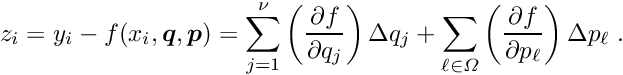
Basic data elements are single measurements ; several single measurements belong to a group of measurements, which can be called a local-fit object. For example in a track-based alignment based on tracks a track is a local-fit object (see section Application: Alignment of tracking detectors for a detailed discussion on the data for tracks in a track-based alignment). A local-fit object is described by a linear or non-linear function $f(x_i,\Vek{q},\Vek{p})$ , depending on a (small) number of local parameters $\Vek{q}$ and in addition on global parameters $\Vek{p}$ :

(12)

$\begin{equation*} \label{eq:measy} y_i = f(x_i,\Vek{q},\Vek{p}) + \varepsilon_i \; . \end{equation*}$

The parameters $\Vek{q}$ are called the local parameters, valid for the specific group of measurements (local-fit object). The quantity $\varepsilon$ is the measurement error, expected to have (for ideal parameter values) mean zero (i.e. the measurement is unbiased) and standard deviation $\sigma_i$ ; often $\varepsilon$ will follow at least The quantity is assumed to be the coordinate of the measured value , and is one of the arguments of the function $f(x_i,\Vek{q},\Vek{p})$ .

The global parameters needed to compute the expectation $f(x_i,\Vek{q},\Vek{p})$ are usually already quite accurate and only small corrections habe to be determined. The convention is often to define the vector $\Vek{p}$ to be a correction with initial values zero. In this case the final values of the global parameters will be small.

The fit of a local-fit object. The local parameters are usually determined in a least squares fit within the users code, assuming fixed global parameter values $\Vek{p}$ . If the function $f(x_i,\Vek{q},\Vek{p})$ depends non-linearly on the local parameters $\Vek{q}$ , an iterative procedure is used, where the function is linearized, i.e. the first derivatives of the function $f(x_i,\Vek{q},\Vek{p})$ with respect to the local parameters $\Vek{q}$ are calculated. Then the function is expressed as a linear function of local parameter corrections $\Vek{\D q}$ at some reference value $\Vek{q}_k$ :

$\begin{equation*} f(x_i,\Vek{q}_k +\Vek{\D q},\Vek{p}) = f(x_i,\Vek{q}_k,\Vek{p}) + \frac{\partial f}{\partial q_1} \D q_1 + \frac{\partial f}{\partial q_2} \D q_2 + \ldots \; , \end{equation*}$

where the derivatives are calculated for $\Vek{q} \equiv \Vek{q}_k$ . The corrections are determined by the linear least squares method, a new reference value is obtained by

$\begin{equation*} \Vek{q}_{k+1} = \Vek{q}_k + \Vek{\D q} \end{equation*}$

and then, with increased by 1, this is repeated until convergence is reached, i.e. until the corrections become essentially zero. For each iteration a linear system of equations (normal equations of least squares) has to be solved for the parameter corrections $\Vek{\D q}$ with a right-hand side vector $\Vek{b}$ with components

$\begin{equation*} b_j= \sum_i \left( \frac{\partial f_i}{\partial q_j} \right) \, \left( y_i - f(x_i,\Vek{q}_k,\Vek{p}_k) \right) \frac{1}{\sigma_i^2} \; , \end{equation*}$

where the sum is over all measurements of the local-fit object. All components become essential zero after convergence.

After convergence the equation (12) can be expressed with the fitted parameters $\Vek{q}$ in the form

$\begin{equation*} y_i = f(x_i,\Vek{q},\Vek{p}) + \frac{\partial f}{\partial q_1} \D q_1 + \frac{\partial f}{\partial q_2} \D q_2 + \ldots + \varepsilon_i \; . \end{equation*}$

The difference $z_i = y_i - f(x_i,\Vek{q},\Vek{p})$ is called the residual and the equation can be expressed in terms of the residual measurement as

(13)

$\begin{equation*} \label{eq:zdef} z_i \equiv y_i - f(x_i,\Vek{q},\Vek{p}) = \left( \frac{\partial f}{\partial q_1} \right) \D q_1 + \left( \frac{\partial f}{\partial q_2} \right) \D q_2 + \ldots + \varepsilon_i \; . \end{equation*}$

After convergence of the local fit all corrections $\D q_1, \, \D q_2, \ldots$ are zero, and the residuals are small and can be called the measurement error. As mentioned above the model function $f(x_i,\Vek{q},\Vek{p})$ may be a linear or a non-linear function of the local parameters. The fit procedure in the users code may be a more advanced method than least squares. In track fits often Kalman filter algorithms are applied to treat effects like multiple scattering into account. But for any fit procedure the final result will be small residuals , and it should also be possible to define the derivatives ${\partial f}/{\partial q_j}$ and ${\partial f}/{\partial p_{\ell}}$ ; these derivatives should express the change of the residual , if the local parameter or the global parameter $p_{\ell}$ is changed by $\D q_j$ or $\D p_{\ell}$ . In a track fit with strong multiple scattering the derivatives will become rather small with increasing track length, because the information content is reduced due to the multiple scattering.

Local fits are later (in Pede) repeated in a simplified form; these fits need as information the difference and the derivatives, and correspond to the last iteration of the local fit, because only small parameter changes ares involved. Modified values of global parameters $\Vek{p}$ during the global fit result in a change of the value of $f(x_i,\Vek{q},\Vek{p})$ and therefore of , which can be calculated from the derivatives. The derivatives with respect to the local parameters allow to repeat the local fit and to calculate corrections for the local parameters $\Vek{q}$ .

Global parameters

Now the global parameters $\Vek{p}$ are considered. The calculation of the residuals $z_i = y_i - f(x_i,\Vek{q},\Vek{p})$ depends on the global parameters $\Vek{p}$ (valid for all local-fit objects). This dependence can be considered in two ways. As expressed above, the parametrization $f(x_i,\Vek{q},\Vek{p})$ depends on the global parameters $\Vek{p}$ and on corrections $\Vek{\D p}$ of the global parameters (this case is assumed below in the sign of the derivatives with respect to the global parameters). Technically equivalent is the case, where the measured value is calculated from a raw measured value, using global parameter values; in this case the residual could be written in the form $z_i = y_i(\Vek{p}) - f(x_i,\Vek{q})$ . It is assumed that reasonable values are already assigned to the global parameters $\Vek{p}$ and the task is to find (small) corrections $\Vek{\D p}$ to these initial values.

Equation (13) is extended to include corrections for global parameters. Usually only few of the global parameters influence a local-fit object. A global parameter carries a label $\ell$ , which is used to identify the global parameter uniquely, and is an arbitrary positive integer. Assuming that labels $\ell$ from a set $\Omega$ contribute to a single measurement the extended equation becomes

(14)

$\begin{equation*} \label{eq:zdefex} z_i = y_i - f(x_i,\Vek{q},\Vek{p}) = \sum_{j=1}^{\nu} \left( \frac{\partial f}{\partial q_j} \right) \D q_j + \sum_{\ell \in \Omega} \left( \frac{\partial f}{\partial p_{\ell}} \right) \D p_{\ell} \; . \end{equation*}$

Millepede essentially performs a fit to all single measurements for all groups of measurements simultaneously for all sets of local parameters and for all global parameters. The result of this simultaneous fit are optimal corrections $\Vek{\D p}$ for all global parameters; there are no limitations in the number of local parameters sets. Within this global fit the local fits (or better: the last iteration of the local fit) has to be repeated for each local-fit object.

Global parameter labels. The label $\ell$ , carried by a global parameter, is an arbitrary positive (31-bit) integer (most-significant bit is zero), and is used to identify the global parameter uniquely. Arbitrary gaps between the numerical values of labels values are allowed. It is recommended to design the label in a way which allows to reconstruct the meaning of the global parameter from the numerical value of the label $\ell$ .

Writing data files with Mille

The user has to provide the following data for each single measurement:

$\begin{alignat*}{2} n_{lc} &= \; \textrm{number of local parameters} & \quad \quad &\textrm{array}: \; \left( \frac{\partial f}{\partial q_j}\right) \\ n_{gl} &= \; \textrm{number of global parameters} & \quad \quad &\textrm{array}: \left( \frac{\partial f}{\partial p_{\ell}}\right) ; \; \textrm{label-array} \quad \ell \\ z &= \; \textrm{residual} \quad \left( \equiv y_i - f(x_i,\Vek{q},\Vek{p}) \right) & \quad \quad &\sigma = \; \textrm{standard deviation of the measurement} \end{alignat*}$

These data are sufficient to compute the least squares normal equations for the local and global fits. Using calls of MILLE the measured data and the derivatives with respect to the local and global parameters are specified; they are collected in a buffer and written as one record when one local-fit object is finished in the user reconstruction code.

Calls for Fortran version: Data files should be written with the Fortran MILLE on the system used for Pede; otherwise the internal file format could be different.

         CALL MILLE(NLC,DERLC,NGL,DERGL,LABEL,RMEAS,SIGMA)

where

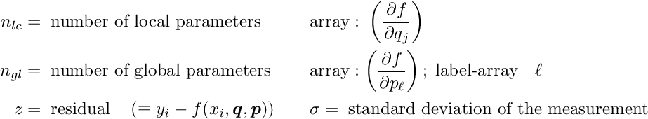
NLC number of local parameters DERLC
DERLC array DERLC(NLC) of derivatives
NGL number of global derivatives in this call
DERGL array DERLG(NGL) of derivatives
LABEL array LABEL(NGL) of labels
RMEAS measured value
SIGMA error of measured value (standard deviation)

After transmitting the data for all measured points the record containing the data for one local-fit object is written. following call

         CALL ENDLE

The buffer content is written to a file with the record.

Alternatively the collected data for the local-fit object have to be discarded, if some reason for not using this local-fit object is found.

         CALL KILLE

The content of the buffer is reset, i.e. the data from preceeding MILLE calls are removed.

Additional floating-point and integer data (special data) can be added to a local fit object by the call

         CALL MILLSP(NSPEC,FSPEC,ISPEC)

where

NSPEC number of special data DERLC
FSPEC array FSPEC(NSPEC) of floating point data
ISPEC array ISPEC(NSPEC) of integer data

The floating-point and integer arrays have the same length. These special data are not yet used, but may be used in future options.

Calls for C version: The C++-class Mille can be used to write C-binary files. The constructor

    Mille(const char *outFileName, bool asBinary = true, bool writeZero = false);

takes at least one argument, defining the name of the output file. For debugging purposes it is possible to give two further arguments: If asBinary is false, a text file (not readable by pede) is written instead of a binary output. If writeZero is true, derivatives that are zero are not suppressed in the output as usual.

The member functions

    void mille(int NLC, const float *derLc, int NGL, const float *derGl,
               const int *label, float rMeas, float sigma);
    void special();
    void end();
    void kill();

have to be called equivalently like the Fortran subroutines MILLE, MILLSP, ENDLE} and KILLE. To properly close the output file, the Mille object should be deleted (or go out of scope) after the last processed record.

Root version: A root version is perhaps added in the future.

Non-linearities

Experience has shown that non-linearities in the function $f(x_i,\Vek{q},\Vek{p})$ are usually small or at least not-dominating. As mentioned before, the convention is often to define the start values of the global parameters as zero and to expect only small final values. Derivatives with respect to the local and global parameters can be assumed to be constants within the range of corrections in the determination of the global parameter corrections. Then a single pass through the data, writing data files and calculating global parameter corrections with Millepede is sufficient. If however corrections are large, they may require to re-calculate the derivatives and another pass or several passes through the data with re-writing data files may be necessary. As a check of the whole procedure a second pass is recommended.

Application: Alignment of tracking detectors

In the alignment of tracking detectors the group of measurement, the local-fit object, may be the set of hits belonging to a single track. Two to five parameters $\Vek{q}$ may be needed to describe the dependence of the measured values on the coordinate .

In a real detector the trajectory of a charged particle does not follow a simple parametrization because of effects like multiple scattering due to the detector material. In practice often a Kalman filter method is used without an explicit parametrization; instead the calculation proceeds along the track taking into account e.g. multiple scattering effects. Derivatives with respect to the (local) track parameters are not directly available. Nevertheless derivatives as required in equation (14) are still well-defined and can be calculated. Assuming that the (local) track parameters refer to the starting point of the track, for each point along the track the derivative $(\partial f/\partial q_j)$ has to be equal to $\D z_i/\D q_j$ , if the local parameter if changed by $\D q_j$ , and the corresponding change of the residual is $\D z_i$ . This derivative could be calculated numerically.

For low-momentum tracks the multiple-scattering effects are large. Thus the derivative above will tend to small values for measured points with a lot of material between the measured point and the starting point of the track. This shows that the contribution of low-momentum tracks with large multiple-scattering effects to the precision of an alignment is small.

Text files

In text files the steering information for the program execution and further information on parameters and constraints is given. The main text file is mandatory. Its default name is steer.txt; if the name is different it has to be given in the command line of Pede. In the main text file the file names of data files and optionally of further text files are given. Text files should have an extension which contains the character pairs xt or tx. In this section all options for the global fits and their keywords are explained. The computation of the global fit is described in detail in the next section Computation of the global fit; it may be necessary to read this section Computation of the global fit to get an understanding of the various options.

General data format of text files

Text files contain file names, numerical data, keywords (text) and comment in free format, but there are certain rules.

File names for all text and steering file should be the leading information in the main steering file, with one file name per line, with correct characters, since the file names are used to open the files.

Numerical can be given with or without decimal point, optionally with exponent field. The numerical data

 13234       13234.0      13.234E+3

are all identical.

Comments can be given in every line, preceeded by the ! sign; the text after the ! is ignored. Lines with * or ! in the first columm are considered as comment lines. Blank lines are ignored.

Keywords are necessary for certain data; they can be given in upper or lower case characters. Keywords with few typo errors may also be recognized correctly. The program will stop if a keyword is not recognized.

Below is an example for a steering file:

  Fortranfiles
  !/home/albert/filealign/lhcrun1.11    ! data from first test run
   /home/albert/filealign/lhcrun2.11    ! data from second run
   /home/albert/filealign/cosmics.bin   ! cosmics
   /home/albert/detalign/mydetector.txt ! steering file from previous log file
   /home/albert/detalign/myconstr.txt   ! test constraints

  constraint 0.14       ! numerical value of r
  713 1.0               ! pair of parameter label and numerical factor
  719 0.5  720 0.5      ! two pairs

  CONSTRAINTS 1.2
   112 1.0
   113 -1.0
   114 0.5
   116 -0.5

  Parameter
  201 0.0   -1.0
  202 1.0   -1.0
  204 1.23 0.020

  method inversion 5 0.1
  end

File information

Names of data and text files are given in single text lines. The file-name extension is used to distinguish text files (extension containing tx or xt) and binary data files. Data files may be Fortran or C files; by default C files are assumed. Fortran files have to be preceded by the textline

   Fortranfiles

and C files may be preceded by the textline

   Cfiles

Mixing of C- and Fortran-files is allowed.

Parameter information

By default all global parameters appearing in data files with their labels are assumed to be variable parameters with initial value zero, and used in the fit. Initial values different from zero and the so-called presigma (see below) may be assigned to global parameters, identified by the parameter label. The optional parameter information has to be provided in the form below, starting with a line with the keyword Parameter:

   Parameter
   label   initial_value   presigma
    ...
   label   initial_value   presigma

The three numbers label, initial_value and presigma in a textline may be followed by further numbers, which are ignored.

Note: Note that the result file has the same format and may be used as input file, if a program execution should be continued.

All parameters not given in this file, but present in the data files are assumed to be variable, with initial value of zero.

Pre-sigma. The pre-sigma $s_{\ell}$ defines the status of the global parameter:

$\boldsymbol{s_{\ell} > 0}$ : The parameter is variable with the given initial value. A term $1/s_{\ell}^2$ is added to the diagonal matrix element of the global parameter to stabilize a perhaps poorly defined parameter. This addition should not bias the fitted parameter value, if a sufficient number of iterations is performed; it may however bias the calculated error of the parameter (this is available only for the matrix inversion method).

$\boldsymbol{s_{\ell} = 0}$ : The pre-sigma is zero; the parameter is variable with the given initial value.

$\boldsymbol{s_{\ell} < 0}$ : The pre-sigma is negative. The parameter is defined as fixed; the initial value of the parameter is used in the fits.

The lines below show examples, with the numerical value of the label, the initial value, and the pre-sigma:

  11 0.01232  0.0    ! parameter variable, non-zero initial value
  12 0.0      0.0    ! parameter variable, initial value zero
  20 0.00232  0.0300 ! parameter variable with initial value 0.00232
  30 0.00111  -1.0   ! parameter fixed, but non-zero parameter value

Result file. At the end of the Pede program a result file millepede.res with the result is written. In the first three columns it carries the label, the fitted parameter value (initial value + correction) and the pre-sigma (default is zero). This file can, perhaps after editing, be used for a repeated Pede job. Column 4 contains the correction and in the case of solution by inversion or diagonalization column 5 its error and optionally column 6 the global correlation.

Constraint information

Equality constraints allow to fix certain undefined or weakly defined linear combinations of global parameters by the addition of equations of the form

$\begin{equation*} c = \sum_{\ell \in \Omega} f_{\ell} \cdot p_{\ell} \end{equation*}$

The constraint value is usually zero. The format is:

   Constraint   value
   label        factor
    ...
   label        factor

where value, label and factor are numerical values. Note that no error of the value is given. The equality constraints are, within the numerical accuracy, exactly observed in a global fit. Each constraint adds another Lagrange multiplier to the problem, and needs the corresponding memory space in the matrix.

Instead of the keyword Constraint the keyword Wconstraint can be given (this option is not yet implemented!). In this case the factor for each global parameter given in the text file is, in addition, multiplied by the weight $W_{\ell}$ of the corresponding global parameter in the complete fit:

$\begin{equation*} c = \sum_{\ell \in \Omega} f_{\ell} \cdot W_{\ell} \cdot p_{\ell} \end{equation*}$

Thus global parameters with a large weight in the fit get also a large weight in the constraint.

Mathematically the effect of a constraint does not change, if the constraint equation is multiplied by an arbitrary number. Because of round-off errors however it is recommended to have the constraint equation on a equal accuracy level, perhaps by a scale factor for constraint equations.

Global parameter measurements

Measurements with measurement value and measurement error for linear combinations of global parameters in the form

$\begin{equation*} y = \sum_{\ell \in \Omega} f_{\ell} \cdot p_{\ell} + \epsilon \end{equation*}$

can be given, where $\epsilon$ is the measurement error, assumed to follow a distribution $N(0,\sigma^2)$ , i.e. zero bias and standard deviation $\sigma$ . The format is:

   Measurement    value    sigma
   label    factor
    ...
   label    factor

where value, sigma, label and factor are numerical values. Each measurement value $\pm$ sigma (standard deviation) given in the text files contributes to the overall objective function in the global fit. At present no outlier tests are made.

The global parameter measurement and the constraint information from the previous section differ, in the definition, only in the additional information on the standard deviation given for the measurement. They differ however in the mathematical method: constraints add another parameter (Lagrange multiplier); measurements contribute to the parameter part of the matrix, and may require no extra space; however a sparse matrix may become less sparse, if matrix elements are added, which are empty otherwise.

Solution method selection

Methods. One out of several solution methods can be selected. The methods have different execution time and memory space requirement, and may also have a slighly different accuracy. The statement to select a method are:

   method inversion         number1 number2
   method diagonalization   number1 number2
   method fullGMRES         number1 number2
   method sparseGMRES       number1 number2
   method cholesky          number1 number2
   method bandcholesky      number1 number2
   method HIP               number1 number2

The two numbers are:

number1 = number of iterations
number2 = limit for $\D F$ (convergence recognition).

For preconditioning in the GMRES methods a band matrix is used. The width of the variable-band matrix is defined by

   bandwidth     number

where number is the numerical value of the semi-bandwidth of a band matrix. The method called bandcholesky uses only the band matrix (reduced memory space requirement), and needs more iterations. The different methods are described below.

Iterations and convergence. The mathematical method in principle allows to solve the problem in a single step. However due to potential inaccuracies in the solution of the large linear system and due to a required outlier treatment certain internal iterations may be necessary. Thus the methods work in iterations, and each iteration requires one or several loops with evaluation of the objective function and the first-derivative vector of the objective function (gradient), which requires reading all data and local fits of the data. The first loop is called iteration 0, and (only) in this loop in addition the second-derivative matrix is evaluated, which takes more cpu time. This first loop usually brings a large reduction of the value of the objective function, and all following loops will bring small additional improvements. In all following loops the same second-derivative matrix is used (in order to reduce cpu time), which should be a good approximation.

A single loop may be sufficient, if there are no outlier problems. Using the command line option $\bf -s$ (subito) the program executes only a single loop, irrespective of the options required in the text files. The treatment of outliers turns a linear problem into a non-linear problem and this requires iterations. Also precision problems, with rounding errors in the case of a large number of global parameters, may require iterations. Each iteration $1, \, 2, \ldots$ is a line search along the calculated search direction, using the strong Wolfe conditions, which force a sufficient decrease of the function value and the gradient. Often an iteration requires only one loop. If, in the outlier treatment, a cut is changed, or if the precision of the constraints is insufficient, one additional loop may be necessary.

At present the iterations end, when the number specified with the method is reached. For each loop, the expected objective-function decrease and the actual decrease are compared. If the two values are below the limit for $\D F$ specified with the method, the program will end earlier.

Memory space requirements. The most important consumer of space is the symmetric matrix of the normal equations. This matrix has a parameter part, which requires for example for full storage words, and for sparse storage words, for number of global parameters and fraction of non-zero off-diagonal elements. In addition the matrix has a constraint part, corresponding to the Lagrange multipliers. Formulae to calculate the number of (double precision) elements of the matrix are given in table 1.

The GMRES method can be used with a full or with a sparse matrix. Without preconditioning the GMRES method may be slow or may even fail to get an acceptable solution. Preconditioning is recommended and usually speeds up the GMRES method considerably. The band matrix required for preconditioning also takes memory space. The parameter part requires (only) $n \cdot m$ words, where semibandwidth specified with the method. A small value like is usually sufficient. The constraint part of the band matrix however requires up to $n \cdot n_C + n_C (n_C+1)$ words, and this can be a large number for large number of constraint equations.

Another matrix with words is required for the constraints, and this matrix is used to improve the precision of the constraints. Several vectors of length and are used in addition, but this space is only proportional to and .

The diagonalization method requires more space: in addition to the symmetric matrix another matrix with words is used for the eigenvectors; since diagonalization is also slower, the method can only be used for smaller problems.

Table 1

Comparison of the methods. The methods have a different computing-time dependence on the number of parameters . The methods diagonalization, inversion and cholesky have a computing time proportional to the third power of n, and can therefore be used only up to 1000 or perhaps up to 5000. Especially the diagonalization is slow, but provides a detailed information on weakly- and well-defined linear combinations of global parameters.

The GMRES methods has a weaker dependence on , and allows much larger -values; larger values of of course require a lot of space and the sparse matrix mode should be used. The bandcholesky method can be used for preconditioning the GMRES method (recommended), but also as a stand-alone method; its cpu time depends only linearly on , but the matrix is only an approximation and usually many iterations are required. For all methods the constraints increase the time and space consumption; this remains modest if the number of constraints is modest, for example $n_C \le 100$ , but may be large for several thousand.

Solution methods

Inversion. The computing time for inversion is roughly $2 \times 10^{-8} \cdot n^3$ seconds (on a standard PC). For 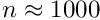$n \approx 1000$ the inversion time of $\approx 20$ seconds is still acceptable, but for $n \approx 10000$ the inversion time would be already more than 5 hours. The advantage of the inversion is the availability of all parameter errors and global correlations.

Cholesky decomposition. The Cholesky decomposition (under test) is an alternative to inversion; eventually this method is faster and/or numerically more stable than inversion. At present parameter errors and global correlations are not available.

Diagonalization. The computing time for diagonalization is roughly a factor 10 larger than for inversion. Space for the square (non-symmetric) transformation matrix of eigenvectors is necessary. Parameter errors and global correlations are calculated for all parameters. The main advantage of the diagonalization method is the availability of the eigenvalues. Small positive eigenvalues of the matrix correspond to linear combinations of parameters which are only weakly defined and it will become possible to interactively remove the weakly defined linear combinations. This removal could be an alternative to certain constraints. Constraints are also possible and they should correspond to negative eigenvalues.

Generalized minimization of residuals (GMRES). The GMRES method is a fast iterative solution method for full and sparse matrices. Especially for large dimensions with $n \gg$ 1000 it should be much faster than inversion, but of similar accuracy. Although the solution is fast, the building of the sparse matrix may require a larger cpu time. At present there is a limit for the number of internal GMRES-iterations of 2000. For a matrix with a bad condition number this number of 2000 internal GMRES-iterations will often be reached and this is often also an indication of a bad and probably inaccurate solution. An improvement is possible by preconditioning, selected if GMRES is selected together with a bandwidth parameter for a band matrix; an approximate solution is determined by solving the matrix equation with a band matrix within the GMRES method, which improves the eigenvalue spectrum of the matrix and often speeds up the method considerably. Experience shows that a small bandwidth of e.g. 6 is sufficient. In interactive mode parameter errors for selected parameters can be determined.

Variable band matrix. Systems of equations with a band matrix can be solved by the Cholesky decomposition. Often the matrix element around the diagonal are the essential matrix elements and in these cases the matrix can be approximated by a band matrix of small width, with a small memory requirement. The computing time is also small; it is linear with the number of parameters. However because the band matrix is only the approximate matrix often many iterations are necessary to get a good solution. The definition of the band width is necessary. The band width is variable and thus the constraints equations can be treated completely. This means that the constraints are observed even in this approximate solution.

Outlier treatment and debugging

Cases with very large residuals within the data can distort the result of the least squares fit. Reason for outliers may be selection mistakes or statistical fluctuations. A good outlier treatment may be neccessary to get accurate results. The problem of outlier treatment is complicated by the fact that initially the global parameters may be far from optimal and therefore large deviation may occur even for correct data before the global parameter determination. There are options for the complete removal of bad cases and for the down-weighting of bad data. Cases with a huge $\chi^2$ are automatically removed in every iteration. The options to remove large $\chi^2$ cases and down-weighting are not done in the first iteration. The options are:

   chisqcut              number1 number2
   outlierdownweighting  number
   dwfractioncut         number
   printrecord           number1 number2

Chisquare cut. With the keyword chisqcut two numbers can be given. Basis of $\chi^2$ rejection is the $\chi^2$ -value corresponding to 3 standard deviations (and to a probability of $0.27 \%$ ). or one degree of freedom this $\chi^2$ -value is 9.0, and for 10 degrees of freedom the $\chi^2$ -value is 26.9. The first number given with the keyword chisqcut is a factor for the $\chi^2$ -cut value, to be used in the first iteration, and the second number is the factor for the second iteration. In subsequent iterations the factor is reduced by the square root, with values below 1.5 replaced by 1. For example the statement

   chisqcut 5.0 2.5

means: the cut factor is $5 \times \chi^2$ -value corresponding to three standard deviations, $2.5 \times \chi^2$ -value for the second iteration, $1.58 \times \chi^2$ -value for the third iteration and $1 \times \chi^2$ -value for subsequent iterations. Thus in the first iteration the cut is $5 \times 26.9 = 134.5$ for 10 degrees of freedom, and after the third iteration.

Outlier downweighting. Outlier down-weighting for single data values requires repeated local fits with iterations in the local fit. The number given with the keyword outlierdownweighting is the number of iterations. In down-weighting the weight of the data point, which by default is $1/\sigma^2$ , is reduced by an extra factor $\omega_i < 1$ according to the residual (see below). For data points the total sum $S_f = \sum_i \omega_i$ of the extra factors is $\le n$ . The ratio is called the down-weight fraction, and a histogram of this ratio is accumulated in the second function evaluation. The first iteration of the local fit is done without down-weighting, iterations 2 and 3 use the M-estimation method with the Huber function. Subsequent iterations, if requested, use the M-estimation method with the Cauchy function for down-weighting, where the influence of very large deviations is further reduced. For example the statement

   outlierdownweighting 4

means: iteration 1 of the local fit without down-weighting, iterations 2 and 3 with Huber function down-weighting and iteration 4 with Cauchy function down-weighting.

Downweighting fraction cut. Cases with a very large fraction of down-weighted measurements are very likely wrong data and should be rejected. The cut value should be determined from the histogram showing the down-weight fraction. Typical values are 0.1 for weights from the Huber function (outlierdownweighting $\le 3$ ) and 0.2 for weights from the Cauchy function (outlierdownweighting ). For example the statement

   dwfractioncut 0.2

means to reject all cases with a down-weight fraction $\ge 0.2$ .

Record printout. For debugging many details of single records and the local fits are printed. Two record number number1 number2 can be given with the keyword printrecord; printout is done in iteration 1 and 3. For numbers given as negative, the records with extreme deviations are selected in iteration 2, and printed in iteration 3. If the first number is given as , the record with the largest single residual is selected. If the second number is given as , the record with the largest value of $\chi^2/N_{df}$ is selected. For example the statement

   printrecord 4321 -1

means: the record 4321 is printed in iterations 1 and 3, and the record with the largest value of $\chi^2/N_{df}$ is selected in iteration 2 and printed in iteration 3.

Further options

There are miscellaneous further options which can be selected within the text files:

   subito
   entries           number
   nofeasiblestart
   wolfe             C1 C2
   histprint
   end

The option subito is also selected by -s in the command line. The program will end regularly, with normal output of the result, already after the first function evaluation (iteration 0).

The number, given with the keyword entries, is the minimum number of data for a global parameter. Global parameters which have a number of entries number of measured points connected to it in the local fit-objects, smaller then the given number are ignored. This option is used to suppress global parameters with only few data, which are therefore rather inaccurate, and would spoil the condition of the linear system.

By default the initial global parameter values are corrected to follow all the constraints. A check for the validity of the constraints is repeated in every iteration, and eventually another correction is made at the end of an iteration. With the keyword nofeasiblestart the parameters are not made feasible (respecting the constraints) at the start.

The constants C1 and C2 are the line search constants for the strong Wolfe conditions; default values are the standard values $C_1 = 10^{-4}$ and .

Histograms accumulated during the program are written to the textfile millepede.his and can be read after the job execution. If selected by the keyword histprint the histograms accumulated during the program are also printed.

The reading of a textfile ends, when the keyword end is encountered. Textlines after the line with end are not read.

Computation of the global fit

Memory managament

The solution of the optimization problem for a large number of parameters requires one large memory with many arrays, required to store vectors and matrices of large size corresponding to the number of parameters and constraints. Millepede II uses a large array in a common. This large array is dynamically divided into so-called subarrays, which are created, enlarged and moved, and removed according to the requirements. The space limitation is thus given for almost all subproblems only by the total space requirement. The largest space is required for the symmetric matrix of the normal least squares equations. This matrix can be a full matrix or for certain problems a sparse matrix. As an approximation a band matrix with a small band width can be used, if there is not enough space for the full or sparse matrix.

Initialization

After initialization of the memory management the command line options are read and analysed. Then the main text file is analysed, the names of other text files and the data files are recognized and stored in a table. Default value are assigned to the various variables; then all text files are read and the requested options are interpreted. The data for the definition for parameters, constraints and measurement are read and stored in subarrays.

First data loop

In subroutine LOOP1 tables for the variable and fixed global parameters and translation tables are defined. The table of global parameter labels is first filled with the global parameters, appearing in the text files. All data files are read and all global parameter labels from the records are included in the list.

There are three integers to characterize a global parameter.

Global parameter label = ITGBL: this is a positive integer, from the full range of 32-bit integers. $1 \ldots 2147483647= 2^{31} -1$ .

Global parameter index = ITGBL: A translation table is constructed to translate the global parameter label ITGBL to a global parameter index ITGBI, with a range $1 \ldots$ NTGB, where NTGB is the total number of global parameters (variable and fixed parameters).

Variable-parameter index = IVGBI: the global parameters which are variable carry a variable-parameter index, with a range $1 \ldots$ NVGB, where NVGB is the number of variable global parameters. Parameter vectors in the mathematical computation are vectors containing only the variable parameters.

Function calls are used to translate the global parameter label ITGBL:

$\begin{alignat*}{2} \textrm{global parameter index} &\leftarrow \textrm{global parameter label} & \quad \quad \quad \texttt{ITGBI} &= \texttt{INONE(ITGBL)} \\ \textrm{variable parameter index} &\leftarrow \textrm{global parameter label} & \quad \quad \quad \texttt{IVGBI} &= \texttt{INSEC(ITGBL)} \; . \end{alignat*}$

The translation is done with a hash-index table. The translation from one parameter index to another one and back to the parameter label is done by the following statement functions:

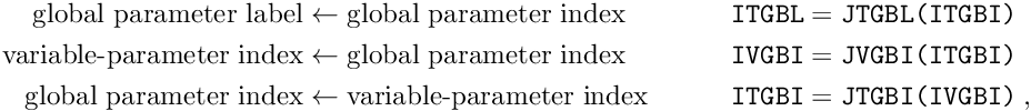
$\begin{alignat*}{2} \textrm{global parameter label} &\leftarrow \textrm{global parameter index} & \quad \quad \quad \texttt{ITGBL} &= \texttt{JTGBL(ITGBI)} \\ \textrm{variable-parameter index} &\leftarrow \textrm{global parameter index} & \quad \quad \quad \texttt{IVGBI} &= \texttt{JVGBI(ITGBI)} \\ \textrm{global parameter index} &\leftarrow \textrm{variable-parameter index} & \quad \quad \quad \texttt{ITGBI} &= \texttt{JTGBI(IVGBI)} \; , \end{alignat*}$

which use simple fixed-length tables.

Second data loop

In subroutine LOOP2 the subarray dimensions of the various vectors and matrices are determined. All data files are read and for each local-fit object the number of local and of global parameters is determined; the maximum values of the numbers are used to define the subarray dimensions for the arrays to be used in local fits, and for the contributions to the global fit.

The sparse matrix storage requires to establish the pointer structure of the sparse matrix. During reading the data files the list of global parameters used in each local-fit object is determined; an entry is made in a table for each pair of global parameters, which later corresponds to an off-diagonal matrix element. A hash-index table is used for the search operation. For sparse and full matrix storage the requirements of the constraint equations and Lagrange multipliers has to be included. For the sparse matrix a pointer structure is build, which allows a fast matrix $\times$ *vector* product. At the end of the subroutine all subarrays required for the determination of the solution are prepared.

Solution method overview

The section gives an short overview over the solution method; more detailed explanation is given in the subsequent sections.

In principle the solution can be determined in a single step; this mode can be selected by the keyword subito or option -s. There are however two reasons to perform iterations, which improve the result:

Due to the large size or the method the one-step solution may be affected by rounding errors and may not be precise. Experience shows that the overall value objective-function value can be reduce using more than one step, although the decrease is sometimes rather small;
Outliers may be important; they add a *non-linear component to the otherwise linear problem and this requires iterations and repeated evaluation of the objective function; each function evaluation requires to read again all data files and to repeat the local fits. In a comparison of Millepede I and II results initially certain differences were observed; only after a careful outlier treatment these differences became small or disappeared.

The solution determined in iterations is explained. The starting iteration, with iteration number 0, is the most important and time-consuming one. The data files are read, and for each case a local fit is made. The matrix of the normal equations is formed only in this starting iteration. Depending on the selected method the matrix is inverted, diagonalized or decomposed, and the resulting matrix and decomposition is used in all later data-file loops, which take less time compared to the first data-file loop. Thus the data-file loop in iteration number 0 may be rather time consuming, especially for the case of a sparse matrix, where the index determination takes some time. The right-hand-side vector is formed in each data-file loop. A correction step in global parameter space is calculated at the end of the data-file loop in iteration number 0. Often the precision is already sufficient and no further data-file loops are necessary. In the subito mode (keyword subito or option -s) the correction is added to the global parameter values and the program stops.

Iterations with more data-file loops are recommended, to check the result, eventually to improve the result and to treat outliers. In each iterations a so-called line search is done, where the overall value of the objective functions is optimized along the correction-step direction sufficiently, using the strong Wolfe criterion. Often a single step is already sufficient for an iteration. The sample of local-fit objects may change during the iterations becuse of changing cut values; this may require extra function and derivative calculations.

Data file loops during iterations

In subroutine LOOPN all data files are read. For each local-fit object the local fit is performed, based on the actual global parameter corrections, and eventually including downweighting of outliers. Using the results of the local fit the value of the objective function , the vector of first derivatives (gradient) and, in the first data file loop, the matrix of second derivatives is calculated. For a linear fit the matrix of second derivatives will not change during the iterations; the outlier treatment will change the matrix, but usually the changes are small und the matrix collected in the first data loop is at least a good and sufficiently accurate approximation. Thus data loops after the first one are faster; depending on the method the solution of the matrix equation will be faster after the first data loop.

The local fit

The number of local parameters of a local-fit object is usually small; typical values are between 2 and 5. Since the problem is linear, a single step is sufficient in a local fit with minimization of the sum

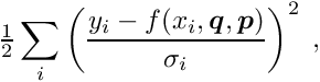
$\begin{equation*} \tfrac{1}{2} \sum_i \left( \frac{y_i - f(x_i,\Vek{q},\Vek{p})}{\sigma_i} \right)^2 \; , \end{equation*}$

unless outlier downweighting is required, which may require a few iterations. In a loop over the local measurements the matrix and the right-hand side of the least squares normal equations are summed. For each single measured value, the residual measurement

$\begin{equation*} z_i \equiv y_i - f(x_i,\Vek{q},\Vek{p}) \end{equation*}$

(see equation (13)) has to be corrected for the actual global parameters corrections $\Vek{\D p}$ using the first global parameter derivatives (see equation (14)). The corrected residual is then used in the accumulation of the matrix and vector:

$\begin{equation*} \Gamma_{jk} = \sum_i \left( \frac{\partial f_i}{\partial q_j} \right) \left( \frac{\partial f_i}{\partial q_k} \right) \frac{1}{\sigma_i^2} \quad \quad \quad \quad \beta_j= \sum_i \left( \frac{\partial f_i}{\partial q_j} \right) \, \frac{z_i'}{\sigma_i^2} \; . \end{equation*}$

Corrections $\Vek{\D q}$ are determined by the solution of the matrix equation

$\begin{equation*} \Vek{\Gamma} \Vek{\D q} = - \Vek{\beta} \; , \end{equation*}$

which is determined using matrix inversion $\Vek{\D q} = - \Vek{\Gamma}^{-1} \Vek{b}$ , because the inverse matrix $\Vek{\Gamma}^{-1}$ (the covariance matrix) is necessary for the contribution to the matrix of the global normal equations. The residual are then corrected for the local parameter corrections:

$\begin{equation*} z_i^{''} = z_i^{'} - \sum_j \frac{\partial f_i}{\partial q_j} \D q_j \end{equation*}$

and the new residuals $z_i^{''}$ are used to calculate the $\chi^2$ value of the local fit

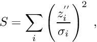
$\begin{equation*} S = \sum_i \left( \frac{z_i^{''}}{\sigma_i} \right)^2 \; , \end{equation*}$

which should follow a $\chi^2$ . The number of local parameters of a local-fit object is usually small; typical values are between 2 and 5. Since the problem is linear, a single step is sufficient in a local fit with minimization of the sum

$\begin{equation*} \tfrac{1}{2} \sum_i \left( \frac{y_i - f(x_i,\Vek{q},\Vek{p})}{\sigma_i} \right)^2 \; , \end{equation*}$

unless outlier downweighting is required, which may require a few iterations. In a loop over the local measurements the matrix and the right-hand side of the least squares normal equations are summed. For each single measured distribution with the given number of degrees of freedom $n_{\textrm{df}} =$ number of measurements minus number of parameters. A fraction of 0.27 % or one out of 370 of the correct cases should have a deviation which corresponds to 3 standard devations in the $n_{\textrm{df}} =1$ case.

Very badly fitting cases should be rejected before using them for the global parameter fit. Basis of the rejection is the comparison of the sum and the 0.27 % value $\chi^2_{\textrm{cut}}$ of the $\chi^2_{n_{\textrm{df}}}$ distribution. If the value exceeds $\chi^2_{\textrm{cut}}$ by more than a factor of 50, then the sum is called huge and the local-fit object is rejected. Cases with $n_{\textrm{df}} =0$ are rejected too, because they do no allow any check. These rejections are always made, even if the user has not requested any outlier rejection.

With keyword chisqcut the user can require a further rejection. The first number given with the keyword is used during iteration 0; the local-fit object is rejected, if the value is larger than this number times $\chi^2_{\textrm{cut}}$ . Often this number has to rather high, e.g. 12.0; the initial value of may be rather high before the first determination of global parameters, even for correct data, and, if possible, no correct data should be rejected by the cut. The second number given with the keyword is used during iteration 1 and can be smaller than the first number, because the first improvement of the local parameters is large. In further iterations the number is reduced by the sqrt-function. Values below 1.5 are replaced by 1, and thus the rejection is finally be done with a 0.27 %-rejection probability for correct data.

All not rejected local-fit objects contribute to the global fit. The function value is the sum of the -values for the local-fit objects:

$\begin{equation*} F = \sum_{l} S_{l} \quad \quad \quad \textrm{sum with index $l$ over all local fit-objects} \; . \end{equation*}$

Here even -values from local-fit objects, which are rejected by cuts are included, with $S_{l} =$ cut value, in order to keep the sum meaningful (otherwise the rejection of many local-fit object could simulate an improvement – which is not the case).

Contributions to the global parameter fit

After an accepted local fit the contributions to the normal least squares equations of the global fit have to be calculated. The first contribution is from the first order derivatives with respect to the global parameters:

(15)

$\begin{equation*} \label{eq:c1} \left(\Vek{\D C}_1\right)_{jk} = \sum_i \left( \frac{\partial f_i}{\partial p_j} \right) \left( \frac{\partial f_i}{\partial p_k} \right) \frac{1}{\sigma_i^2} \quad \quad \quad \quad \D g_j= \sum_i \left( \frac{\partial f_i}{\partial p_j} \right) \, \frac{z_i^{''}}{\sigma_i^2} \; . \end{equation*}$

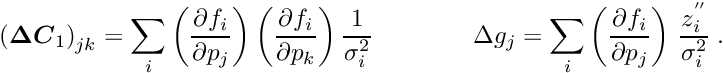
Note that in the -term the residual is already corrected for the local fit result. The vector $\Vek{g}$ is the gradient of the global objective function.

The second contribution is, according to the Millepede principle, a mixed contribution from first order global and local derivatives. After the local fit the matrix $\Vek{G}$ is formed, which has a number of columns equal to the number of local parameters, and a number of rows equal to the number of global parameters. The elements are

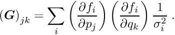
$\begin{equation*} \left(\Vek{G}\right)_{jk} = \sum_i \left( \frac{\partial f_i}{\partial p_j} \right) \left( \frac{\partial f_i}{\partial q_k} \right) \frac{1}{\sigma_i^2} \; . \end{equation*}$

The second contribution to the global matrix $\Vek{C}$ is then

(16)

$\begin{equation*} \label{eq:c2} \Vek{\D C_2} = - \Vek{G} \Vek{\Gamma}^{-1} \Vek{G}\trans \end{equation*}$

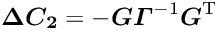
with the matrices $\Vek{G}$ and $\Vek{\Gamma}$ from a local fit. Because of the dimension of matrices $\Vek{G}$ and $\Vek{\D C}$ the calculation would require a large number of operations. However only a small number of rows of matrix $\Vek{G}$ is not equal to zero and the calculation can be restricted, with the help of pointers, to the non-zero part and in addition one can use the fact that the result is a symmetric matrix. With this code, which may appear somewhat complicated in comparison to the standard matrix multiplication, the computation time is small. Note that no extra contribution to the gradient vector $\Vek{g}$ is necessary because the residual $z_i^{''}$ used above already includes the local fit result. The sum $\Vek{C}$ of the two contributions, $\Vek{\D C}_1$ from equation (15), and $\Vek{\D C}_2$ from equation (16), summed over all local fit-objects, is the final matrix of the least squares normal equations. Element $(\Vek{C})_{jk}$ is related to the global parameters with indices and . The matrix $\Vek{C}$ corresponds to a simultaneous fit of the global and local parameters of all local-fit objects. The first term (15) alone corresponds to the fit, when the local parameters are assumed to be fixed; only those elements $(\Vek{C})_{jk}$ of the matrix $\Vek{C}$ are non-zero, where the two global parameters with indices and appear in the same measurement . In contrast, in the second term (16) those elements $(\Vek{C})_{jk}$ of the matrix $\Vek{C}$ are non-zero, where the two global parameters with indices and appear in the same local fit.

Outlier downweighting in local fits

The influence of a single measurement resp. is proportional to the absolute value of the normalised residual $\zeta_i = z_i/\sigma_i$ in the pure least squares fit of local-fit objects. Thus measurements with a large deviation will in general distort the resulting fit. This effect can be avoided by downweighting those measurements. Measurements with large residuals are included in the method of M-estimates by assigning to them, instead of the ideal Gaussian distribution of least squares, a different distribution with larger tails. Technically this is done by multiplying the standard weight $1/\sigma_i^2$ of least squares by another factor, which depends on the actual value of $\zeta_i = z_i/\sigma_i$ . This method requires an initial fit without downweighting, followed by iterative downweighting.

In Millepede II the local fits are improved, if necessary, by downweighting after the first iteration, with a number of iterations specified by the user with keyword outlierdownweighting {it numberofiterations}. In iterations 2 and 3 the downweighting is done with the Huber function and the Cauchy function is used, if more iterations are requested (see section Outlier treatment and debugging for an explanation of the two functions).

Global fit

Global fit without constraints

The aim is to find a step vector $\Vek{\D p}$ , which minimizes the objective function: $F(\Vek{p} + \Vek{\D p}) =$ minimum. In the -th iteration the approximate solution is $\Vek{p}_k$ . A quadrative model function $\widetilde{F}(\Vek{p} + \Vek{d})$

(17)

$\begin{equation*} \label{eq:quadapp} \widetilde{F}(\Vek{p}_k + \Vek{d} ) = F_k + \Vek{g}\trans \Vek{d} + \tfrac{1}{2} \Vek{d}\trans \Vek{C} \Vek{d} \end{equation*}$

is defined with a vector $\Vek{d}$ . The step vector $\Vek{d}$ is determined as solution of the linear system

$\begin{equation*} \label{eq:stepd} \Vek{C} \Vek{d} = - \Vek{g} \; . \end{equation*}$

The step $\Vek{d}$ will minimize the quadratic function $\widetilde{F}(\Vek{p} + \Vek{d})$ of equation (17), unless there is some inaccuracy due to rounding errors and other approximations of the matrix or the solution method. In order to get a sufficient decrease of the objective function $F(\Vek{p} + \Vek{\D p})$ a line search algorithm is used.

Line search

In the line search algorithm a search is made for the minimum of the function $F(\Vek{p} + \Vek{\D p})$ along a line $\Vek{p} + \alpha \cdot \Vek{d}$ in the parameter space, where $\alpha$ is a factor to be determined. A function $\Phi(\alpha)$ of this factor,

$\begin{equation*} \Phi(\alpha) \equiv F(\Vek{p} + \alpha \cdot \Vek{d}) \end{equation*}$

is considered. Each function evaluation at a certain value of $\alpha$ requires one loop through the data with all local fits. The function value for $\alpha=0$ is already calculated before (start value); the first value of $\alpha$ to be considered is $\alpha=1$ and this value is often already a sufficiently accurate minimum. In the line search algorithm the so-called strong Wolfe conditions are used; these are

$\begin{align*} F( \Vek{p} + \alpha \cdot \Vek{d}) & \le F( \Vek{p}) + C_1 \alpha \nabla F\trans \Vek{d} \\ \left| \nabla F(\Vek{p} + \alpha \cdot \Vek{d})\trans \Vek{d} \right| & \le C_2 \left| \nabla F\trans \Vek{d} \right| \end{align*}$

with . The first condition requires a sufficient decrease of the function. The second condition, called curvature condition, ensures a slope reduction, and rules out unacceptable short steps. In practice the constant is chosen to small, for example $C_1 = 10^{-4}$ . Typical values of the constant are 0.9 for a search vector by a Newton method and 0.1 for a search vector by the conjugate gradient method. Default values in Millepede II are $C_1 = 10^{-4}, \, C_2 = 0.9$ . Often only one value of $\alpha$ , sometimes two to three values are evaluated. The last function value should never be higher than the start value.

Iterations

The global fit can be performed with a result $\Vek{\D p}$ in one step, if the matrix equation is accurately solved and if there are no outliers. The result $\Vek{\D p}$ calculated in the first data loop is usually already close to the final solution; it gives the largest reduction of the objective function. Outliers introduce some non-linearity into the problem and require iterations with repeated data loops. Another argument for repeating the steps is the non-neglectigible inaccuracy of the numerical solution of the step calculation due to rounding errors for the large number of parameters.

Iteration 0. The first data loop is called iteration 0. The function value, the first derivative vector $\Vek{g}$ and the second derivative matrix $\Vek{C}$ or an approximation to it are calculated. They allow to calculate the first step $\Vek{\D p}= \Vek{d}$ .

Iteration $\ge 1$ . In all further iterations a line search is performed. Starting value is the point in parameter space, obtained in the previous iteration. Each function evaluation requires a data loop with local fits. The expected decrease $\D F$ in an iteration can be estimated by

$\begin{equation*} \D F_{\textrm{estimate}} = - \Vek{g}\trans \Vek{d} \; . \end{equation*}$

This can be compared with the actual decrease

$\begin{equation*} \D F_{\textrm{actual}} = F(\Vek{p}) - F(\Vek{p}+ \alpha \Vek{d}) \end{equation*}$

at the end of the iteration. Both values should become smaller during the iterations; convergence can be assumed if both are of the order of $\approx 1$ .

Global fit with constraints

In the Lagrange multiplier method one additional parameter $\lambda$ is introduced for each single constraint, resulting in an -vector $\Vek{\lambda}$ of Lagrange multiplier. A term depending on $\Vek{\lambda}$ and the constraints is added to the objective function, resulting in the Lagrange function

$\begin{equation*} \mathcal{L}(\Vek{p},\Vek{\lambda}) = F_k + \Vek{g}\trans \Vek{d} + \tfrac{1}{2} \Vek{d}\trans \Vek{C} \Vek{d} + \Vek{\lambda} \left( \Vek{A} \left( \Vek{p}_k + \Vek{d}\right) - \Vek{c} \right) \end{equation*}$

Using as before a quadratic model for the function $F(\Vek{p})$ and taking derivatives w.r.t. the parameters $\Vek{p}$ and the Lagrange multipliers $\Vek{\lambda}$ , the two equations

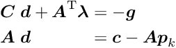
$\begin{alignat*}{2} \Vek{C} \; & \Vek{d} + \Vek{A}\trans & \Vek{\lambda} & = - \Vek{g} \\ \Vek{A} \; & \Vek{d} & & = \Vek{c} - \Vek{A} \Vek{p}_k \end{alignat*}$

are obtained; the second of these equations is the constraint equation. This system of two equations can be combined into one matrix equation

$\begin{equation*} \label{eq:lageq} \left( \begin{array}{ccc|c} & & & \\ & \Vek{C} & & \Vek{A}\trans \\ & & & \\ \hline & \Vek{A} & & \Vek{0} \end{array} \right) \left( \begin{array}{c} ~\\ \Vek{d} \\ ~\\ \hline \lambda \end{array} \right) = \left( \begin{array}{c} ~\\ - \Vek{g} \\ ~\\ \hline \Vek{c} - \Vek{A} \Vek{p}_k \end{array} \right) \; . \end{equation*}$

The matrix on the left hand side is still symmetric. Linear least squares problems with linear constraints can be solved directly, without iterations and without the need for initial values of the parameters. Insufficient precision of the equality constraints is corrected by the method discussed in section Feasible parameters.

Output text files

Several output text file are generated in Pede. All files have a fixed name. If files with this name are existing at the Pede start, they are renamed by appending a $\sim$ to the file name; existing files with file name already carrying the $\sim$ are removed!

Log-file for Pede. The file millepede.log summarizes the job execution. Especially information on the iterations is given.

Result file. The file millepede.res contains one line per (variable or fixed) global parameter; the first three numbers have the same meaning as the lines following the Parameter keyword in the input text files. The first value is the label, the second is the fitted parameter value, and the third is the presigma, either copied from the input text file or zero (default value).

Debug file. The file mpdebug.txt, if requested by the printrecord keyword, contains detailed information of all data and fits for local-fit objects.

Eigenvector file. The file millepede.eve is written for the method diagonalization. It contains selected eigenvectors and their eigenvalues, and can be used e.g. for an analysis of weak modes.

Using Millepede II for track based alignment

Global parameters

Global parameters to be determined in a track-based alignment are mostly geometrical corrections like translation shifts and rotation angles. Usually only small corrections to the default position and angle information are necessary, and the assumption of constant first derivatives is sufficient (otherwise an iteration with creation of new data files would be necessary). In general an alignment should be done simultaneously of all relevant detectors, perhaps using structural constraints (see below).

In addition to the geometrical corrections there are several additional parameters, which determine track-hit positions like Lorentz-angle and -values, drift-velocities etc. These parameters should be included in the alignment process, since, due to the correlation between all pairs of global parameters, a separate determination of those parameters cannot be optimal. Also beam parameters like vertex position and beam direction angles should be included in the alignment, if those value are used with the tracks. Incorrectness of the model used e.g. to calculate the expected track hit positions, for example a wrong value of the Lorentz-angle, can introduce distortions in other parameters.

Constraints

Equality constraints are, in the mathematical sense, equations between global parameters, which have to be exact (within the computing accuracy). Only linear constraints are supported. Below two areas of constraints are discussed.

Removal of undefined degrees of freedom

A general linear transformation has 12 parameters. Three parameters of the translation and additional three parameters of a rotation are undefined, if only track residuals are minimized. At least these six parameters have to be fixed by constraining to zero the overall translation and rotation.

Structural constraints

A large track detector has usually a sub-detector structure: the track detector is built from smaller units, which are built by smaller sub-units etc. down to the level of a single sensor. The different levels can be visualized by a tree structure. Figure 2 shows the tree structure of the cms detector.

The tree structure can be reflected in the label structure and constraints. One set of global parameters is assigned to a unit. To each of the subunits another set of global parameters; the sum of the transformations of the subunits is forced to zero by sum constraints, which remove the otherwise undefined degrees of freedom. For a unit with subunits, with for example 6 degrees of freedom, the total number of degrees of freedom becomes

$\begin{equation*} \left[ 6 + 6 \cdot N \right] \; \textrm{(parameters)} - 6 \; \textrm{(constraints)} = 6 \cdot N \; . \end{equation*}$

The parameters of the unit are more accurately defined than the parameters of the sub-units. Additional external measurement information from e.g. a survey can be assigned to the parameters of the unit. If all sub-unit parameters are fixed after an initial alignment, the parameters of the unit can still be variable and be improved in an alignment with a reduced total number of parameters.

Figure 2

Figure 2: The tree of components of the cms inner track detectors.

Linear transformations in 3D

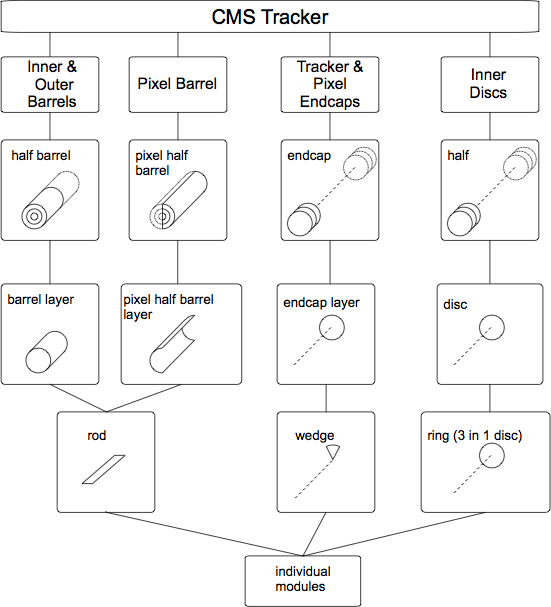
Nominal transformation. For track reconstruction the local coordinate system and the global $x \, y \,z$ coordinate system are used. The local system with coordinate $\Vek{q}$ and components , and is defined w.r.t. a sensor with origin at the center of the sensor; the -axis is along the precise and the -axis is along the coarse coordinate, and the -axis is normal to the sensor. The transformation from the global to the local system is given by

$\begin{equation*} \Vek{q} = \Vek{R} \left( \Vek{r} - \Vek{r}_0 \right) \end{equation*}$

with the definitions

$\begin{equation*} \Vek{q} = \left( \begin{array}{c} u \\ v \\ w \end{array} \right) \quad \quad \quad \Vek{r} = \left( \begin{array}{c} x \\ y \\ z \end{array} \right) \quad \quad \quad \Vek{r}_0 = \left( \begin{array}{c} x_0 \\ y_0 \\ z_0 \end{array} \right) \; . \end{equation*}$

The nominal position $\Vek{r}_0$ and the rotation matrix $\Vek{R}$ are determined by detector assembly and survey information. The convention is to use the three Euler angles $\vartheta$ , $\psi$ and $\varphi$ to determine the nominal rotation matrix $\Vek{R}$ :

$\begin{equation*} \Vek{R} = \left( \begin{array}{ccc} \cos \psi \, \cos \varphi - \cos \vartheta \, \sin \psi \, \sin \varphi & - \cos \psi \, \sin \varphi - \cos \vartheta \, \sin \psi \, \cos \varphi & \sin \vartheta \, \sin \psi \\ \sin \psi \, \cos \varphi + \cos \vartheta \, \cos \psi \, \sin \varphi & - \sin \psi \, \sin \varphi + \cos \vartheta \, \cos \psi \, \cos \varphi & - \sin \vartheta \, \cos \psi \\ \sin \vartheta \, \sin \varphi & \sin \vartheta \, \cos \varphi & \cos \vartheta \end{array} \right) \end{equation*}$

or

$\begin{equation*} \Vek{R} = \left( \begin{array}{ccc} \cos \psi \, \cos \varphi - \cos \vartheta \, \sin \psi \, \sin \varphi & \sin \psi \, \cos \varphi + \cos \vartheta \, \cos \psi \, \sin \varphi & \sin \vartheta \, \sin \varphi \\ - \cos \psi \, \sin \varphi - \cos \vartheta \, \sin \psi \, \cos \varphi & - \sin \psi \, \sin \varphi + \cos \vartheta \, \cos \psi \, \cos \varphi & \sin \vartheta \, \cos \varphi \\ \sin \vartheta \, \sin \psi & - \sin \vartheta \, \cos \psi & \cos \vartheta \end{array} \right) \end{equation*}$

The ranges of the angles are: $0 \le \vartheta < \pi$ , $0 \le \psi < 2 \pi$ , and $0 \le \phi < 2 \pi$ .

A different convention is to parametrize the rotation by Euler angles $\varphi$ , $\vartheta$ and $\psi$ with the rotation $\Vek{R} = \Vek{R}_3(\varphi) \Vek{R}_2(\vartheta) \Vek{R}_3(\psi)$ , where $R_i(\delta)$ is a rotation by an angle $\delta$ about the axis $\Vek{n}_i$ . The rotation is

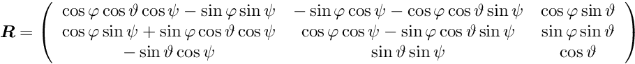
$\begin{equation*} \Vek{R} = \left( \begin{array}{ccc} \cos \varphi \cos \vartheta \cos \psi - \sin \varphi \sin \psi & -\sin \varphi \cos \psi - \cos \varphi \cos \vartheta \sin \psi & \cos \varphi \sin \vartheta \\ \cos \varphi \sin \psi + \sin \varphi \cos \vartheta \cos \psi & \cos \varphi \cos \psi - \sin \varphi \cos \vartheta \sin \psi & \sin \varphi \sin \vartheta \\ -\sin\vartheta \cos \psi & \sin \vartheta \sin \psi & \cos \vartheta \end{array} \right) \end{equation*}$

The ranges of the angles are: $0 \le \phi < 2 \pi$ , $0 \le \vartheta < \pi$ and $0 \le \psi < 2 \pi$ .

Alignment correction to the transformation. The alignment procedure determines a correction to the nominal transformation by an incremental rotation $\D \Vek{R}$ and a translation $\D \Vek{r}_0$ . The combined translation and rotation becomes

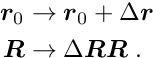
$\begin{align*} \Vek{r}_0 &\to \Vek{r}_0 + \D \Vek{r} \\ \Vek{R} &\to \D \Vek{R} \Vek{R} \; . \end{align*}$

The correction matrix $\D \Vek{R}$ is given by small rotations by $\D \alpha$ , \, $\D \beta$ and $\D \gamma$ around the -axis, the (new) -axis and the (new) -axis:

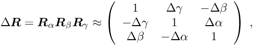
$\begin{equation*} \D \Vek{R} = \Vek{R}_{\alpha} \Vek{R}_{\beta} \Vek{R}_{\gamma} \approx \left( \begin{array}{ccc} 1 & \D \gamma & - \D \beta \\ - \D \gamma & 1 & \D \alpha \\ \D \beta & - \D\alpha & 1 \end{array} \right) \; , \end{equation*}$

where the approximation has sufficient accuracy for small angles $\D \alpha$ , \, $\D \beta$ and $\D \gamma$ . The position correction $\D \Vek{r}$ transforms to the local system as

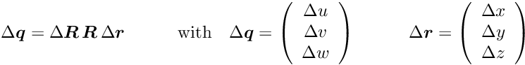
$\begin{equation*} \D \Vek{q} = \D \Vek{R} \, \Vek{R} \, \D \Vek{r} \quad \quad \quad \textrm{with} \quad \D \Vek{q} = \left( \begin{array}{c} \D u \\ \D v \\ \D w \end{array} \right) \quad \quad \quad \D \Vek{r} = \left( \begin{array}{c} \D x \\ \D y \\ \D z\end{array} \right) \end{equation*}$

These corrections define the corrected (aligned) transformation from global to local coordinates:

$\begin{equation*} \Vek{q}^{\textrm{aligned}} = \D \Vek{R} \, \Vek{R} \left( \Vek{r} - \Vek{r}_0 \right) - \D \Vek{q} \; . \end{equation*}$

The task of the alignment by tracks is to determine the correction angles $\D \alpha$ , $\D \beta$ and $\D \gamma$ (and thus the rotation matrix $\D \Vek{R}$ ) and the translation vector $\D \Vek{r}$ or vector $\D \Vek{q}$ for each individual detector element.

Acknowledgement

Markus Stoye has worked with different versions of Millepede II during the development phase in the last two years in alignment studies for the inner tracker of the cms experiment. I would like to thank him for the close collaboration, which was essential for the development of Millepede II. I would like to thank also Gero Flucke, who contributed the C $^{++}$ code, and Claus Kleinwort for the Millepede I/II comparison using data from the H1 experiment.

Table of Contents

Preface

Mathematical Methods

Large problems with global and local parameters

Optimization without constraints

The quadratic model

Partitioning of matrices

Local parameters

Global parameters

The simultaneous fit of global and local parameters

Reduction of matrix size

Nonlinear least squares

Outliers

Optimization with linear constraints

The Lagrange multiplier method

Feasible parameters

The Manual

The programm package Millepede II

Program code and makefile

Data collection in the user program with subroutine Mille

Solution with the stand-alone program Pede

Measurements and parameters

Measurements and local parameters

Global parameters

Writing data files with Mille

Non-linearities

Application: Alignment of tracking detectors

Text files

General data format of text files

File information

Parameter information

Constraint information

Global parameter measurements

Solution method selection

Solution methods

Outlier treatment and debugging

Further options

Computation of the global fit

Memory managament

Initialization

First data loop

Second data loop

Solution method overview

Data file loops during iterations

The local fit

Contributions to the global parameter fit

Outlier downweighting in local fits

Global fit

Global fit without constraints

Line search

Iterations

Global fit with constraints

Output text files

Using Millepede II for track based alignment

Global parameters

Constraints

Removal of undefined degrees of freedom

Structural constraints

Linear transformations in 3D

Acknowledgement